Concept Check ✅ – Answer at cc.dsc10.com
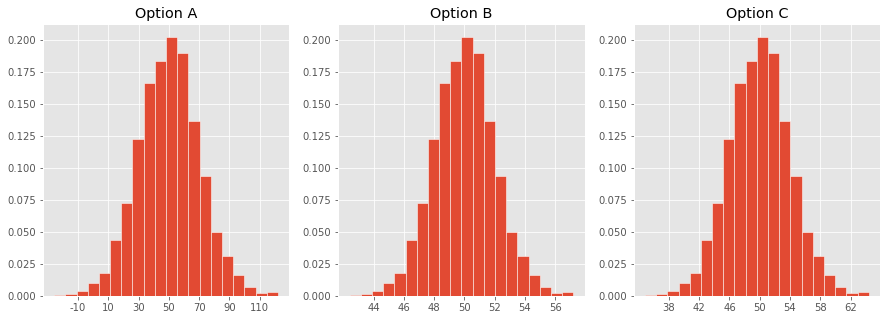
Which one of these histograms corresponds to the distribution of the sample mean for samples of size 100 drawn from a population with mean 50 and SD 20?
# Set up packages for lecture. Don't worry about understanding this code, but
# make sure to run it if you're following along.
import numpy as np
import babypandas as bpd
import pandas as pd
from matplotlib_inline.backend_inline import set_matplotlib_formats
import matplotlib.pyplot as plt
from scipy import stats
set_matplotlib_formats("svg")
plt.style.use('ggplot')

np.set_printoptions(threshold=20, precision=2, suppress=True)
pd.set_option("display.max_rows", 7)
pd.set_option("display.max_columns", 8)
pd.set_option("display.precision", 2)

# Animations
from IPython.display import display, IFrame, HTML
import ipywidgets as widgets

def normal_curve(x, mu=0, sigma=1):
    return 1 / np.sqrt(2*np.pi) * np.exp(-(x - mu)**2/(2 * sigma**2))

def normal_area(a, b, bars=False, title=None):
    x = np.linspace(-4, 4)
    y = normal_curve(x)
    ix = (x >= a) & (x <= b)
    plt.plot(x, y, color='black')
    plt.fill_between(x[ix], y[ix], color='gold')
    if bars:
        plt.axvline(a, color='red')
        plt.axvline(b, color='red')
    if title:
        plt.title(title)
    else:
        plt.title(f'Area between {np.round(a, 2)} and {np.round(b, 2)}')
    plt.show()

def area_within(z):
    title = f'Proportion of values within {z} SDs of the mean: {np.round(stats.norm.cdf(z) - stats.norm.cdf(-z), 4)}'
    normal_area(-z, z, title=title)

def show_clt_slides():
    src = "https://docs.google.com/presentation/d/e/2PACX-1vTcJd3U1H1KoXqBFcWGKFUPjZbeW4oiNZZLCFY8jqvSDsl4L1rRTg7980nPs1TGCAecYKUZxH5MZIBh/embed?start=false&loop=false&delayms=3000"
    width = 960
    height = 509
    display(IFrame(src, width, height))
show_clt_slides()
Let's draw one sample then bootstrap to generate 2000 resample means.
np.random.seed(42)
delays = bpd.read_csv('data/delays.csv')
my_sample = delays.sample(500)
resample_means = np.array([])
repetitions = 2000

for i in np.arange(repetitions):
    resample = my_sample.sample(500, replace=True)
    resample_mean = resample.get('Delay').mean()
    resample_means = np.append(resample_means, resample_mean)

resample_means
array([12.65, 11.5 , 11.34, ..., 12.59, 11.89, 12.58])
bpd.DataFrame().assign(resample_means=resample_means).plot(kind='hist', density=True, ec='w', alpha=0.65, bins=20, figsize=(10, 5));
plt.scatter([resample_means.mean()], [-0.005], marker='^', color='green', s=250)
plt.axvline(resample_means.mean(), color='green', label=f'mean={np.round(resample_means.mean(), 2)}', linewidth=4)
plt.xlim(7, 20)
plt.ylim(-0.015, 0.35)
plt.legend();
One approach to computing a confidence interval for the population mean involves taking the middle 95% of this distribution.
left_boot = np.percentile(resample_means, 2.5)
right_boot = np.percentile(resample_means, 97.5)
[left_boot, right_boot]
[10.7159, 15.43405]
bpd.DataFrame().assign(resample_means=resample_means).plot(kind='hist', y='resample_means', alpha=0.65, bins=20, density=True, ec='w', figsize=(10, 5), title='Distribution of Bootstrapped Sample Means');
plt.plot([left_boot, right_boot], [0, 0], color='gold', linewidth=10, label='95% bootstrap-based confidence interval');
plt.xlim(7, 20);
plt.legend();
But we didn't need to bootstrap to learn what the distribution of the sample mean looks like. We could instead use the CLT, which tells us that the distribution of the sample mean is normal. Further, its mean and standard deviation are approximately:
samp_mean_mean = my_sample.get('Delay').mean()
samp_mean_mean
13.008
samp_mean_sd = np.std(my_sample.get('Delay')) / np.sqrt(my_sample.shape[0])
samp_mean_sd
1.2511114546674091
So, the distribution of the sample mean is approximately:
plt.figure(figsize=(10, 5))
norm_x = np.linspace(7, 20)
norm_y = normal_curve(norm_x, mu=samp_mean_mean, sigma=samp_mean_sd)
plt.plot(norm_x, norm_y, color='black', linestyle='--', linewidth=4, label='Distribution of the Sample Mean (via the CLT)')
plt.xlim(7, 20)
plt.legend();
Question: What interval on the $x$-axis captures the middle 95% of this distribution?
As we saw last class, if a variable is roughly normal, then approximately 95% of its values are within 2 standard deviations of its mean.
normal_area(-2, 2)
stats.norm.cdf(2) - stats.norm.cdf(-2)
0.9544997361036416
Let's use this fact here!
my_delays = my_sample.get('Delay')
left_normal = my_delays.mean() - 2 * np.std(my_delays) / np.sqrt(500)
right_normal = my_delays.mean() + 2 * np.std(my_delays) / np.sqrt(500)
[left_normal, right_normal]
[10.50577709066518, 15.510222909334818]
plt.figure(figsize=(10, 5))
norm_x = np.linspace(7, 20)
norm_y = normal_curve(norm_x, mu=samp_mean_mean, sigma=samp_mean_sd)
plt.plot(norm_x, norm_y, color='black', linestyle='--', linewidth=4, label='Distribution of the Sample Mean (via the CLT)')
plt.xlim(7, 20)
plt.ylim(0, 0.41)
plt.plot([left_normal, right_normal], [0, 0], color='#8f6100', linewidth=10, label='95% CLT-based confidence interval')
plt.legend();
We've constructed two confidence intervals for the population mean:
One using bootstrapping,
[left_boot, right_boot]
[10.7159, 15.43405]
and one using the CLT.
[left_normal, right_normal]
[10.50577709066518, 15.510222909334818]
In both cases, we only used information in my_sample, not the population.
The intervals created using each method are slightly different, because there are some approximations involved:
A 95% confidence interval for the population mean is given by
$$ \left[\text{sample mean} - 2\cdot \frac{\text{sample SD}}{\sqrt{\text{sample size}}}, \text{sample mean} + 2\cdot \frac{\text{sample SD}}{\sqrt{\text{sample size}}} \right] $$This CI doesn't require bootstrapping, and it only requires three numbers – the sample mean, the sample SD, and the sample size!
Bootstrapping still has its uses!
| Bootstrap | CLT | |
|---|---|---|
| Pro | Works for many sample statistics (mean, median, standard deviation). |
Only requires 3 numbers – the sample mean, sample SD, and sample size. |
| Con | Very computationally expensive (requires drawing many, many samples from the original sample). |
Only works for the sample mean (and sum). |
We just saw that when $z = 2$, the following is a 95% confidence interval for the population mean.
$$ \left[\text{sample mean} - z\cdot \frac{\text{sample SD}}{\sqrt{\text{sample size}}}, \text{sample mean} + z\cdot \frac{\text{sample SD}}{\sqrt{\text{sample size}}} \right] $$Question: What value of $z$ should we use to create an 80% confidence interval? 90%?
z = widgets.FloatSlider(value=2, min=0,max=4,step=0.05, description='z')
ui = widgets.HBox([z])
out = widgets.interactive_output(area_within, {'z': z})
display(ui, out)
Which one of these histograms corresponds to the distribution of the sample mean for samples of size 100 drawn from a population with mean 50 and SD 20?
temperatures = bpd.read_csv('data/temp.csv')
temperatures
| temperature | |
|---|---|
| 0 | 96.3 |
| 1 | 96.7 |
| 2 | 96.9 |
| ... | ... |
| 127 | 99.9 |
| 128 | 100.0 |
| 129 | 100.8 |
130 rows × 1 columns
temperatures.get('temperature').describe()
count    130.00
mean      98.25
std        0.73
          ...
50%       98.30
75%       98.70
max      100.80
Name: temperature, Length: 8, dtype: float64
The mean body temperature of all people is a population mean!
sample_mean = temperatures.get('temperature').mean()
sample_mean
98.24923076923078
sample_mean_sd = np.std(temperatures.get('temperature')) / np.sqrt(temperatures.shape[0])
sample_mean_sd
0.06405661469519337
# 95% confidence interval for the mean body temperature of all people:
[sample_mean - 2 * sample_mean_sd, sample_mean + 2 * sample_mean_sd]
[98.12111753984038, 98.37734399862117]
Careful! This doesn't mean that 95% of temperatures in our sample (or the population) fall in this range!
plt.figure(figsize=(10, 5))
plt.hist(temperatures.get('temperature'), density=True, bins=20, ec='w');
plt.title('Sample Distribution of Body Temperature (ºF)');
plt.plot([sample_mean - 2*sample_mean_sd, sample_mean + 2*sample_mean_sd], [0, 0], color='gold', linewidth=20, label='95% CLT-based confidence interval')
plt.legend();
# 95% confidence interval for the mean body temperature of all people:
[sample_mean - 2 * sample_mean_sd, sample_mean + 2 * sample_mean_sd]
[98.12111753984038, 98.37734399862117]

Question: How big of a sample do you need? 🤔
Key takeaway: The CLT applies in this case as well! The distribution of the proportion of 1s in our sample is roughly normal.
We will:
Note that the width of our CI is the right endpoint minus the left endpoint:
$$ \text{width} = 4 \cdot \frac{\text{sample SD}}{\sqrt{\text{sample size}}} $$# Plot the SD of a collection of 0s and 1s with p proportion of Os.
p = np.arange(0, 1.01, 0.01)
sd = np.sqrt(p * (1 - p))
plt.plot(p, sd)
plt.xlabel('p')
plt.ylabel(r'$\sqrt{p(1-p)}$');
By substituting 0.5 for the sample size, we get
While any sample size that satisfies the above inequality will give us a confidence interval that satisfies the necessary properties, it's time-consuming to gather larger samples than necessary. So, we'll pick the smallest sample size that satisfies the above inequality.
(4 * 0.5 / 0.06) ** 2
1111.1111111111113
Conclusion: We must sample 1112 people to construct a 95% CI for the population mean that is at most 0.06 wide.
Suppose we instead want an a 95% CI for the population mean that is at most 0.03 wide. What is the smallest sample size we could collect?
Hint: Use the fact that we must sample 1112 people for a 95% CI for the population mean that is at most 0.06 wide.
At a high level, the second half of this class has been about statistical inference – using a sample to draw conclusions about the population.