# Set up packages for lecture. Don't worry about understanding this code,
# but make sure to run it if you're following along.
import numpy as np
import babypandas as bpd
import pandas as pd
from matplotlib_inline.backend_inline import set_matplotlib_formats
import matplotlib.pyplot as plt
set_matplotlib_formats("svg")
plt.style.use('ggplot')

np.set_printoptions(threshold=20, precision=2, suppress=True)
pd.set_option("display.max_rows", 7)
pd.set_option("display.max_columns", 8)
pd.set_option("display.precision", 2)

# Animations
from IPython.display import display, IFrame

def show_bootstrapping_slides():
    src = "https://docs.google.com/presentation/d/e/2PACX-1vS_iYHJYXSVMMZ-YQVFwMEFR6EFN3FDSAvaMyUm-YJfLQgRMTHm3vI-wWJJ5999eFJq70nWp2hyItZg/embed?start=false&loop=false&delayms=3000&rm=minimal"
    width = 960
    height = 509
    display(IFrame(src, width, height))

Lecture 15 – Bootstrapping and Confidence Intervals

DSC 10, Fall 2023

Announcements

• The Midterm Project deadline is pushed back to Monday at 11:59PM.
  • You can still use up to two slip days to extend the deadline further. This will detract from both partners' allocations.
  • Only one partner should submit and "Add Group Member" on Gradescope.
• Lab 4 will be released today and is due Thursday 11/9 at 11:59PM.
• Homework 4 will be released this weekend and is due Saturday 11/11 at 11:59PM.
• Along with Lab 4, we are releasing a Mid-Quarter Survey, which will allow you to give us feedback on the course anonymously. If at least 80% of the class fills it out by Saturday 11/11 at 11:59PM, everyone will earn 2 additional points on the Midterm Exam!

Agenda

• Recap: Statistical inference.
• Bootstrapping 🥾.
• Percentiles.
• Confidence intervals.

Recap: Statistical inference

City of San Diego employee salary data

All City of San Diego employee salary data is public. We are using the latest available data.

population = bpd.read_csv('data/2022_salaries.csv')
population

	Year	EmployerType	EmployerName	DepartmentOrSubdivision	...	EmployerCounty	SpecialDistrictActivities	IncludesUnfundedLiability	SpecialDistrictType
0	2022	City	San Diego	Police	...	San Diego	NaN	False	NaN
1	2022	City	San Diego	Police	...	San Diego	NaN	False	NaN
2	2022	City	San Diego	Fire-Rescue	...	San Diego	NaN	False	NaN
...	...	...	...	...	...	...	...	...	...
12826	2022	City	San Diego	Public Utilities	...	San Diego	NaN	False	NaN
12827	2022	City	San Diego	Police	...	San Diego	NaN	False	NaN
12828	2022	City	San Diego	Police	...	San Diego	NaN	False	NaN

12829 rows × 29 columns

When you load in a dataset that has so many columns that you can't see them all, it's a good idea to look at the column names.

population.columns

Index(['Year', 'EmployerType', 'EmployerName', 'DepartmentOrSubdivision',
       'Position', 'ElectedOfficial', 'Judicial', 'OtherPositions',
       'MinPositionSalary', 'MaxPositionSalary', 'ReportedBaseWage',
       'RegularPay', 'OvertimePay', 'LumpSumPay', 'OtherPay', 'TotalWages',
       'DefinedBenefitPlanContribution', 'EmployeesRetirementCostCovered',
       'DeferredCompensationPlan', 'HealthDentalVision',
       'TotalRetirementAndHealthContribution', 'PensionFormula', 'EmployerURL',
       'EmployerPopulation', 'LastUpdatedDate', 'EmployerCounty',
       'SpecialDistrictActivities', 'IncludesUnfundedLiability',
       'SpecialDistrictType'],
      dtype='object')

We only need the 'TotalWages' column, so let's get just that column.

population = population.get(['TotalWages'])
population

	TotalWages
0	384909
1	381566
2	350013
...	...
12826	6
12827	4
12828	2

12829 rows × 1 columns

population.plot(kind='hist', bins=np.arange(0, 400000, 10000), density=True, ec='w', figsize=(10, 5),
                title='Distribution of Total Wages of San Diego City Employees in 2022');

The median salary

• We can use .median() to find the median salary of all city employees.
• This is a population parameter.
• This is not a random quantity.

population_median = population.get('TotalWages').median()
population_median

78136.0

Let's be realistic...

• In practice, it is costly and time-consuming to survey all 12,000+ employees.
  • More generally, we can't expect to survey all members of the population we care about.
  • We happen to have the population here, but generally we won't.

• Instead, we gather salaries for a random sample of, say, 500 people.

Terminology recap

• The full DataFrame of salaries is the population.

• We observe a sample of 500 salaries from the population.

• We want to determine the population median (a parameter), but we don't have the whole population, so instead we use the sample median (a statistic) as an estimate.

• Hopefully the sample median is close to the population median.

The sample median

Let's survey 500 employees at random. To do so, we can use the .sample method.

np.random.seed(38) # Magic to ensure that we get the same results every time this code is run.

# Take a sample of size 500.
my_sample = population.sample(500)
my_sample

	TotalWages
10301	27866
6913	71861
5163	91843
...	...
3002	121209
3718	109709
2394	131409

500 rows × 1 columns

We won't reassign my_sample at any point in this notebook, so it will always refer to this particular sample.

# Compute the sample median.
sample_median = my_sample.get('TotalWages').median()
sample_median

76237.0

How confident are we that this is a good estimate?

• Our estimate depended on a random sample. If our sample was different, our estimate may have been different, too.

• How different could our estimate have been? Our confidence in the estimate depends on the answer to this question.

• The sample median is a random number. It comes from some distribution, which we don't know.

• If we did know what the distribution of the sample median looked like, it would help us determine how different our estimate might have been, if we'd drawn a different sample.
  • "Narrow" distribution $\Rightarrow$ not too different.
  • "Wide" distribution $\Rightarrow$ quite different.

An impractical approach

• One idea: repeatedly collect random samples of 500 from the population and compute their medians.
  • This is what we did last class, to compute an empirical distribution of the sample mean of flight delays.

sample_medians = np.array([])
for i in np.arange(1000):
    median = population.sample(500).get('TotalWages').median()
    sample_medians = np.append(sample_medians, median)
sample_medians

array([81686.5, 79641. , 75592. , ..., 79350. , 78826.5, 78459.5])

(bpd.DataFrame()
 .assign(SampleMedians=sample_medians)
 .plot(kind='hist', density=True,
       bins=30, ec='w', figsize=(8, 5),
       title='Distribution of the Sample Median of 1000 Samples from the Population\nSample Size = 500')
);

• This shows an empirical distribution of the sample median. It is an approximation of the true probability distribution of the sample median, based on 1000 samples.

The problem

• Drawing new samples like this is impractical – we usually can't just ask for new samples from the population.
  • If we were able to do this, why not just collect more data in the first place?

• Key insight: our original sample, my_sample, looks a lot like the population.
  • Their distributions are similar.

fig, ax = plt.subplots(figsize=(10, 5))
bins=np.arange(10_000, 300_000, 10_000)
population.plot(kind='hist', y='TotalWages', ax=ax, density=True, alpha=.75, bins=bins, ec='w')
my_sample.plot(kind='hist', y='TotalWages', ax=ax, density=True, alpha=.75, bins=bins, ec='w')
plt.legend(['Population', 'My Sample']);

Note that unlike the previous histogram we saw, this is depicting the distribution of the population and of one particular sample (my_sample), not the distribution of sample medians for 1000 samples.

Bootstrapping 🥾

Bootstrapping

• Shortcut: Use the sample in lieu of the population.
  • The sample itself looks like the population.
  • So, resampling from the sample is kind of like sampling from the population.
  • The act of resampling from a sample is called bootstrapping.

• In our case specifically:
  • We have a sample of 500 salaries.
  • We want another sample of 500 salaries, but we can't draw from the population.
  • However, the original sample looks like the population.
  • So, let's just resample from the sample!

show_bootstrapping_slides()

To replace or not replace?

• Our goal when bootstrapping is to create a sample of the same size as our original sample.

• Let's repeatedly resample 3 numbers without replacement from an original sample of [1, 2, 3].

original = [1, 2, 3]
for i in np.arange(10):
    resample = np.random.choice(original, 3, replace=False)
    print("Resample: ", resample, "    Median: ", np.median(resample))

Resample:  [2 1 3]     Median:  2.0
Resample:  [1 2 3]     Median:  2.0
Resample:  [1 2 3]     Median:  2.0
Resample:  [3 1 2]     Median:  2.0
Resample:  [1 3 2]     Median:  2.0
Resample:  [1 3 2]     Median:  2.0
Resample:  [3 1 2]     Median:  2.0
Resample:  [3 2 1]     Median:  2.0
Resample:  [1 2 3]     Median:  2.0
Resample:  [3 2 1]     Median:  2.0

• Let's repeatedly resample 3 numbers with replacement from an original sample of [1, 2, 3].

original = [1, 2, 3]
for i in np.arange(10):
    resample = np.random.choice(original, 3, replace=True)
    print("Resample: ", resample, "    Median: ", np.median(resample))

Resample:  [3 2 1]     Median:  2.0
Resample:  [1 1 3]     Median:  1.0
Resample:  [3 2 1]     Median:  2.0
Resample:  [1 1 2]     Median:  1.0
Resample:  [2 1 3]     Median:  2.0
Resample:  [3 3 3]     Median:  3.0
Resample:  [1 1 1]     Median:  1.0
Resample:  [2 2 3]     Median:  2.0
Resample:  [2 3 2]     Median:  2.0
Resample:  [3 3 2]     Median:  3.0

• When we resample without replacement, resamples look just like the original samples.

• When we resample with replacement, resamples can have a different mean, median, max, and min than the original sample.

• So, we need to sample with replacement to ensure that our resamples can be different from the original sample.

Bootstrapping the sample of salaries

We can simulate the act of collecting new samples by sampling with replacement from our original sample, my_sample.

# Note that the population DataFrame, population, doesn't appear anywhere here.
# This is all based on one sample, my_sample.

n_resamples = 5000
boot_medians = np.array([])

for i in range(n_resamples):
    
    # Resample from my_sample WITH REPLACEMENT.
    resample = my_sample.sample(500, replace=True)
    
    # Compute the median.
    median = resample.get('TotalWages').median()
    
    # Store it in our array of medians.
    boot_medians = np.append(boot_medians, median)

boot_medians

array([75592., 77408., 71970., ..., 80386., 77134., 78893.])

Bootstrap distribution of the sample median

bpd.DataFrame().assign(BootstrapMedians=boot_medians).plot(kind='hist', density=True, bins=np.arange(63000, 88000, 1000), ec='w', figsize=(10, 5))
plt.scatter(population_median, 0.000004, color='blue', s=100, label='population median').set_zorder(2)
plt.legend();

The population median (blue dot) is near the middle.

In reality, we'd never get to see this!

What's the point of bootstrapping?

We have a sample median wage:

my_sample.get('TotalWages').median()

76237.0

With it, we can say that the population median wage is approximately \$76,237, and not much else.

But by bootstrapping our one sample, we can generate an empirical distribution of the sample median:

(bpd.DataFrame()
 .assign(BootstrapMedians=boot_medians)
 .plot(kind='hist', density=True, bins=np.arange(63000, 88000, 1000), ec='w', figsize=(10, 5))
)
plt.legend();

which allows us to say things like

We think the population median wage is between \$68,000 and \\$82,000.

Question: We could also say that we think the population median wage is between \$70,000 and \\$80,000, or between \$65,000 and \\$85,000. What range should we pick?

Percentiles

Informal definition

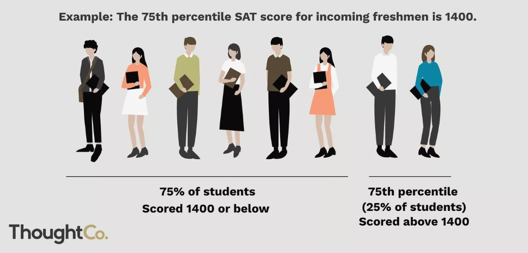
Let $p$ be a number between 0 and 100. The $p$th percentile of a numerical dataset is a number that's greater than or equal to $p$ percent of all data values.

Another example: If you're in the $80$th percentile for height, it means that roughly $80\%$ of people are shorter than you, and $20\%$ are taller.

Calculating percentiles

• The numpy package provides a function to calculate percentiles, np.percentile(array, p), which returns the pth percentile of array.
• We won't worry about how this value is calculated - we'll just use the result!

np.percentile([4, 6, 9, 2, 7], 50)

6.0

np.percentile([2, 4, 6, 7, 9], 50)

6.0

Confidence intervals

Using the bootstrapped distribution of sample medians

Earlier in the lecture, we generated a bootstrapped distribution of sample medians.

bpd.DataFrame().assign(BootstrapMedians=boot_medians).plot(kind='hist', density=True, bins=np.arange(63000, 88000, 1000), ec='w', figsize=(10, 5))
plt.scatter(population_median, 0.000004, color='blue', s=100, label='population median').set_zorder(2)
plt.legend();

What can we do with this distribution, now that we know about percentiles?

Using the bootstrapped distribution of sample medians

• We have a sample median, \$76,237.

• As such, we think the population median is close to \$76,237. However, we're not quite sure how close.

• How do we capture our uncertainty about this guess?

• 💡 Idea: Find a range that captures most (e.g. 95%) of the bootstrapped distribution of sample medians.

Confidence intervals

Let's be a bit more precise.

• Goal: Estimate an unknown population parameter.

• We have been saying:

  We think the population parameter is close to our sample statistic, $x$.

• We want to say:

  We think the population parameter is between $a$ and $b$.

• To do this, we'll use the bootstrapped distribution of a sample statistic to compute an interval that contains "the bulk" of the sample statistics. Such an interval is called a confidence interval.

Finding endpoints

• We want to find two points, $x$ and $y$, such that:
  • The area to the left of $x$ in the bootstrapped distribution is about 2.5%.
  • The area to the right of $y$ in the bootstrapped distribution is about 2.5%.

• The interval $[x,y]$ will contain about 95% of the total area, i.e. 95% of the total values. As such, we will call $[x, y]$ a 95% confidence interval.

• $x$ and $y$ are the 2.5th percentile and 97.5th percentile, respectively.

Computing a confidence interval

boot_medians

array([75592., 77408., 71970., ..., 80386., 77134., 78893.])

# Left endpoint.
left = np.percentile(boot_medians, 2.5)
left

68515.3125

# Right endpoint.
right = np.percentile(boot_medians, 97.5)
right

81505.5

# Therefore, our interval is:
[left, right]

[68515.3125, 81505.5]

You will use the code above very frequently moving forward!

Visualizing our 95% confidence interval

• Let's draw the interval we just computed on the histogram.
• 95% of the bootstrap medians fell into this interval.

bpd.DataFrame().assign(BootstrapMedians=boot_medians).plot(kind='hist', density=True, bins=np.arange(63000, 88000, 1000), ec='w', figsize=(10, 5), zorder=1)
plt.plot([left, right], [0, 0], color='gold', linewidth=12, label='95% confidence interval', zorder=2);
plt.scatter(population_median, 0.000004, color='blue', s=100, label='population median', zorder=3)
plt.legend();

• In this case, our 95% confidence interval (gold line) contains the true population parameter (blue dot).
  • It won't always, because you might have a bad original sample!
  • In reality, you won't know where the population parameter is, and so you won't know if your confidence interval contains it.
• Note that the histogram is not centered around the population median (\$78,136), but it is centered around the sample median (\\$76,237).

Concept Check ✅ – Answer at cc.dsc10.com

We computed the following 95% confidence interval:

print('Interval:', [left, right])
print('Width:', right - left)

Interval: [68515.3125, 81505.5]
Width: 12990.1875

If we instead computed an 80% confidence interval, would it be wider or narrower?

A. Wider                  B. Narrower                  C. Impossible to tell </center

Reflection

Now, instead of saying

We think the population median is close to our sample median, \$76,237.

We can say:

A 95% confidence interval for the population median is \$68,515 to \\$81,505.

Some lingering questions: What does 95% confidence mean? What are we confident about? Is this technique always "good"?

Summary, next time

Summary

• Given a single sample, we want to estimate some population parameter using just one sample. One sample gives one estimate of the parameter. To get a sense of how much our estimate might have been different with a different sample, we need more samples.
  • In real life, sampling is expensive. You only get one sample!
• Key idea: The distribution of a sample looks a lot like the distribution of the population it was drawn from. So we can treat it like the population and resample from it.
• Each resample yields another estimate of the parameter. Taken together, many estimates give a sense of how much variability exists in our estimates, or how certain we are of any single estimate being accurate.
• Bootstrapping gives us a way to generate the empirical distribution of a sample statistic. From this distribution, we can create a $c$% confidence interval by taking the middle $c$% of values of the bootstrapped distribution.
• Such an interval allows us to quantify the uncertainty in our estimate of a population parameter.
  • Instead of providing just a single estimate of a population parameter, e.g. \$76,237, we can provide a range of estimates, e.g. \\$68,515 to \$81,505.
  • Confidence intervals are used in a variety of fields to capture uncertainty. For instance, political researchers create confidence intervals for the proportion of votes their favorite candidate will receive, given a poll of voters.

Next time

We will:

• Give more context to what the confidence level of a confidence interval means, and learn how to interpret confidence intervals.
• Identify statistics for which bootstrapping doesn't work well.
• Quantify the spread of a distribution.