Concept Check ✅ – Answer at cc.dsc10.com
Which one of these histograms corresponds to the distribution of the sample mean for samples of size 100 drawn from a population with mean 50 and SD 20?

# Set up packages for lecture. Don't worry about understanding this code,
# but make sure to run it if you're following along.
import numpy as np
import babypandas as bpd
import pandas as pd
from matplotlib_inline.backend_inline import set_matplotlib_formats
import matplotlib.pyplot as plt
from scipy import stats
set_matplotlib_formats("svg")
plt.style.use('ggplot')

np.set_printoptions(threshold=20, precision=2, suppress=True)
pd.set_option("display.max_rows", 7)
pd.set_option("display.max_columns", 8)
pd.set_option("display.precision", 2)

# Animations
from IPython.display import display, IFrame, HTML
import ipywidgets as widgets

import warnings
warnings.filterwarnings('ignore')

def normal_curve(x, mu=0, sigma=1):
    return 1 / np.sqrt(2*np.pi) * np.exp(-(x - mu)**2/(2 * sigma**2))

def normal_area(a, b, bars=False, title=None):
    x = np.linspace(-4, 4)
    y = normal_curve(x)
    ix = (x >= a) & (x <= b)
    plt.plot(x, y, color='black')
    plt.fill_between(x[ix], y[ix], color='gold')
    if bars:
        plt.axvline(a, color='red')
        plt.axvline(b, color='red')
    if title:
        plt.title(title)
    else:
        plt.title(f'Area between {np.round(a, 2)} and {np.round(b, 2)}')
    plt.show()

def area_within(z):
    title = f'Proportion of values within {z} SDs of the mean: {np.round(stats.norm.cdf(z) - stats.norm.cdf(-z), 4)}'
    normal_area(-z, z, title=title)

def show_clt_slides():
    src = "https://docs.google.com/presentation/d/e/2PACX-1vTcJd3U1H1KoXqBFcWGKFUPjZbeW4oiNZZLCFY8jqvSDsl4L1rRTg7980nPs1TGCAecYKUZxH5MZIBh/embed?start=false&loop=false&delayms=3000&rm=minimal"
    width = 960
    height = 509
    display(IFrame(src, width, height))
show_clt_slides()
A 95% confidence interval for the population mean is given by
$$ \left[\text{sample mean} - 2\cdot \frac{\text{sample SD}}{\sqrt{\text{sample size}}}, \text{sample mean} + 2\cdot \frac{\text{sample SD}}{\sqrt{\text{sample size}}} \right] $$This CI doesn't require bootstrapping, and it only requires three numbers – the sample mean, the sample SD, and the sample size!
Bootstrapping still has its uses!
| Bootstrapping | CLT | |
|---|---|---|
| Pro | Works for many sample statistics (mean, median, standard deviation). |
Only requires 3 numbers – the sample mean, sample SD, and sample size. |
| Con | Very computationally expensive (requires drawing many, many samples from the original sample). |
Only works for the sample mean (and sum). |
We just saw that when $z = 2$, the following is a 95% confidence interval for the population mean.
$$ \left[\text{sample mean} - z\cdot \frac{\text{sample SD}}{\sqrt{\text{sample size}}}, \text{sample mean} + z\cdot \frac{\text{sample SD}}{\sqrt{\text{sample size}}} \right] $$Question: What value of $z$ should we use to create an 80% confidence interval? 90%?
z = widgets.FloatSlider(value=2, min=0,max=4,step=0.05, description='z')
ui = widgets.HBox([z])
out = widgets.interactive_output(area_within, {'z': z})
display(ui, out)
HBox(children=(FloatSlider(value=2.0, description='z', max=4.0, step=0.05),))
Output()
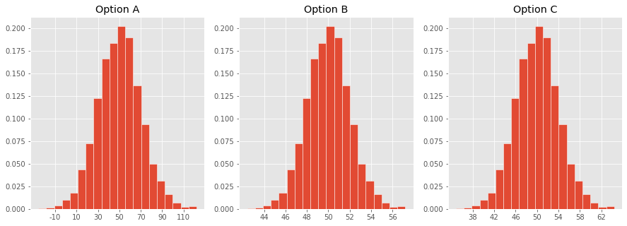
Which one of these histograms corresponds to the distribution of the sample mean for samples of size 100 drawn from a population with mean 50 and SD 20?


Question: How big of a sample do you need? 🤔
Key takeaway: The CLT applies in this case as well! The distribution of the proportion of 1s in our sample is roughly normal.
We will:
Note that the width of our CI is the right endpoint minus the left endpoint:
$$ \text{width} = 4 \cdot \frac{\text{sample SD}}{\sqrt{\text{sample size}}} $$# Plot the SD of a collection of 0s and 1s with p proportion of Os.
p = np.arange(0, 1.01, 0.01)
sd = np.sqrt(p * (1 - p))
plt.plot(p, sd)
plt.xlabel('p')
plt.ylabel(r'$\sqrt{p(1-p)}$');
By substituting 0.5 for the sample size, we get
While any sample size that satisfies the above inequality will give us a confidence interval that satisfies the necessary properties, it's time-consuming to gather larger samples than necessary. So, we'll pick the smallest sample size that satisfies the above inequality.
(4 * 0.5 / 0.06) ** 2
1111.1111111111113
Conclusion: We must sample 1112 people to construct a 95% CI for the population mean that is at most 0.06 wide.
Suppose we instead want an a 95% CI for the population mean that is at most 0.03 wide. What is the smallest sample size we could collect?
A model is a set of assumptions about how data was generated.

"... the overall percentage disparity has been small...”
np.random.choice won't help us, because we don't know how large the eligible population is.np.random.multinomial helps us sample at random from a categorical distribution.np.random.multinomial(sample_size, pop_distribution)
np.random.multinomial samples at random from the population, with replacement, and returns a random array containing counts in each category.pop_distribution needs to be an array containing the probabilities of each category.Aside: Example usage of np.random.multinomial
On Halloween 👻, you trick-or-treated at 35 houses, each of which had an identical candy box, containing:
At each house, you selected one candy blindly from the candy box.
To simulate the act of going to 35 houses, we can use np.random.multinomial:
np.random.multinomial(35, [0.3, 0.3, 0.4])
array([10, 11, 14])
In our case, a randomly selected member of our population is Black with probability 0.26 and not Black with probability 1 - 0.26 = 0.74.
demographics = [0.26, 0.74]
Each time we run the following cell, we'll get a new random sample of 100 people from this population.
np.random.multinomial(100, demographics)
array([22, 78])
We also need to calculate the statistic, which in this case is the number of Black men in the random sample of 100.
np.random.multinomial(100, demographics)[0]
21
counts.counts = np.array([])
for i in np.arange(10000):
new_count = np.random.multinomial(100, demographics)[0]
counts = np.append(counts, new_count)
counts
array([28., 27., 24., ..., 28., 22., 28.])
Was a jury panel with 8 Black men suspiciously unusual?
(bpd.DataFrame().assign(count_black_men=counts)
                .plot(kind='hist', bins = np.arange(9.5, 45, 1),
                      density=True, ec='w', figsize=(10, 5),
                      title='Empiricial Distribution of the Number of Black Men in Simulated Jury Panels of Size 100'));
observed_count = 8
plt.axvline(observed_count, color='black', linewidth=4, label='Observed Number of Black Men in Actual Jury Panel')
plt.legend();
# In 10,000 random experiments, the panel with the fewest Black men had how many?
counts.min()
11.0