In [1]:
# Set up packages for lecture. Don't worry about understanding this code,
# but make sure to run it if you're following along.
import numpy as np
import babypandas as bpd
import pandas as pd
from matplotlib_inline.backend_inline import set_matplotlib_formats
import matplotlib.pyplot as plt
set_matplotlib_formats("svg")
plt.style.use('ggplot')

np.set_printoptions(threshold=20, precision=2, suppress=True)
pd.set_option("display.max_rows", 7)
pd.set_option("display.max_columns", 8)
pd.set_option("display.precision", 2)

# Animations
from IPython.display import display, IFrame

def show_confidence_interval_slides():
    src="https://docs.google.com/presentation/d/e/2PACX-1vTaPZsueXI6fey_5cj2Y1TevkR1joBvpwaWVsZNvgBlnJSrw1EiBLHJywkFH_QNLU5Tdr6JZgDrhFxG/embed?start=false&loop=false&delayms=3000&rm=minimal"
    width = 940
    height = 940
    display(IFrame(src, width, height))

Lecture 20 – Confidence Intervals, Central Tendency

DSC 10, Spring 2023

Announcements

  • Lab 5 is due tomorrow at 11:59PM.
  • Homework 5 is due on Tuesday 5/23 at 11:59PM.
    • See this post on Ed for a few important clarifications.
  • The Final Project is due on Tuesday 6/6 at 11:59PM.
  • The HDSI Undergraduate Scholarship application is due in July! Find a faculty member, propose a project, and if selected, you'll win money to work on your project. See this page for details. All majors are welcome!

Agenda

  • Interpreting confidence intervals.
  • Confidence intervals for hypothesis testing.
  • Central tendency.

Interpreting confidence intervals

Recap: City of San Diego employee salaries

Let's rerun our code from last time to compute a 95% confidence interval for the median salary of all San Diego city employees, based on a sample of 500 people.

Step 1: Collect a single sample of size 500 from the population.

In [2]:
population = bpd.read_csv('data/2021_salaries.csv').get(['TotalWages'])
population_median = population.get('TotalWages').median()
population_median # Can't see this in real life!
Out[2]:
74441.0
In [3]:
np.random.seed(38) # Magic to ensure that we get the same results every time this code is run.
my_sample = population.sample(500)
sample_median = my_sample.get('TotalWages').median()
sample_median
Out[3]:
72016.0

Step 2: Bootstrap! That is, resample from the sample a large number of times, and each time, compute the median of the resample. This will generate an empirical distribution of the sample median.

In [4]:
np.random.seed(38)

# Bootstrap the sample to get more sample medians.
n_resamples = 5000
boot_medians = np.array([])

for i in np.arange(n_resamples):
    resample = my_sample.sample(500, replace=True)
    median = resample.get('TotalWages').median()
    boot_medians = np.append(boot_medians, median)
    
boot_medians
Out[4]:
array([74261. , 73080. , 72486. , ..., 68216. , 76159. , 69768.5])

Step 3: Take the middle 95% of the empirical distribution of sample medians (i.e. boot_medians). This creates our 95% confidence interval.

In [5]:
left = np.percentile(boot_medians, 2.5)
right = np.percentile(boot_medians, 97.5)

# Therefore, our interval is:
[left, right]
Out[5]:
[66987.0, 76527.0]
In [6]:
bpd.DataFrame().assign(BootstrapMedians=boot_medians).plot(kind='hist', density=True, bins=np.arange(60000, 85000, 1000), ec='w', figsize=(10, 5))
plt.plot([left, right], [0, 0], color='gold', linewidth=12, label='95% confidence interval');
plt.scatter(population_median, 0.000004, color='blue', s=100, label='population median').set_zorder(3)
plt.legend();
2023-05-18T21:55:48.017015 image/svg+xml Matplotlib v3.5.2, https://matplotlib.org/

Concept Check ✅ – Answer at cc.dsc10.com

We computed the following 95% confidence interval:

In [7]:
print('Interval:', [left, right])
print('Width:', right - left)
Interval: [66987.0, 76527.0]
Width: 9540.0

If we instead computed an 80% confidence interval, would it be wider or narrower?

A. Wider                  B. Narrower                  C. Impossible to tell </center

Confidence intervals describe a guess for the value of an unknown parameter

Now, instead of saying

We think the population median is close to our sample median, \$72,016.

We can say:

A 95% confidence interval for the population median is \$66,987 to \\$76,527.

Today, we'll address: What does 95% confidence mean? What are we confident about? Is this technique always "good"?

Interpreting confidence intervals

  • We created a confidence interval that contained 95% of our bootstrapped sample medians.
  • We're pretty confident that the true population median does, too.
  • How confident should we be about this? What does a 95% confidence level mean?

Capturing the true value

  • Consider the following three-step process:
    1. Collecting a new original sample from the population.
    2. Bootstrap resampling from it many times, computing the statistic (e.g. median) in each resample.
    3. Constructing a new 95% confidence interval.
  • A 95% confidence level means that approximately 95% of the time, the intervals you create through this process will contain the true population parameter.
  • The confidence is in the process that generates the interval.

Many confidence intervals

  • We repeated the aforementioned process 200 times, to come up with 200 confidence intervals.
    • We did this in advance (it took a really long time) and saved the results to a file.
  • The resulting CIs are stored in the array many_cis below.
In [8]:
many_cis = np.load('data/many_cis.npy')
many_cis
Out[8]:
array([[70247.  , 80075.68],
       [63787.65, 75957.5 ],
       [71493.  , 82207.5 ],
       ...,
       [66679.64, 81308.  ],
       [65735.68, 80060.21],
       [69756.1 , 80383.5 ]])

In the visualization below,

  • The blue line represents the population parameter. This is not random.
  • Each gold line represents a separate confidence interval, created using the specified process.
  • Most of these confidence intervals contain the true parameter – but not all!
In [9]:
plt.figure(figsize=(10, 6))
for i, ci in enumerate(many_cis):
    plt.plot([ci[0], ci[1]], [i, i], color='gold', linewidth=2)
plt.axvline(x=population_median, color='blue');
2023-05-18T21:55:48.342246 image/svg+xml Matplotlib v3.5.2, https://matplotlib.org/

Which confidence intervals don't contain the true parameter?

In [10]:
plt.figure(figsize=(10, 6))
count_outside = 0
for i, ci in enumerate(many_cis):
    if ci[0] > population_median or ci[1] < population_median:
        plt.plot([ci[0], ci[1]], [i, i], color='gold', linewidth=2)
        count_outside = count_outside + 1
plt.axvline(x=population_median, color='blue');
2023-05-18T21:55:48.509714 image/svg+xml Matplotlib v3.5.2, https://matplotlib.org/
In [11]:
count_outside
Out[11]:
11
  • 11 of our 200 confidence intervals didn't contain the true parameter.
  • That means 189/200, or 94.5% of them, did.
    • This is pretty close to 95%!
  • In reality, you will have only one confidence interval, and no way of knowing if it contains the true parameter, since you have no way of knowing if your one original sample is good.

Confidence tradeoffs

  • When we use an "unlucky" sample to make our CI, the CI won't contain the population parameter.
  • If we choose a 99% confidence level,
    • only about 1% of our samples will be "unlucky", but
    • our intervals will be very wide and thus not that useful.
  • If we choose an 80% confidence level,
    • more of our samples will be "unlucky", but
    • our intervals will be narrower and thus more precise.
  • At a fixed confidence level, how do we decrease the width of a confidence interval?
    • By taking a bigger sample!
    • We'll soon see how sample sizes, confidence levels, and CI widths are related to one another.

Misinterpreting confidence intervals

Confidence intervals can be hard to interpret.

In [12]:
# Our interval:
[left, right]
Out[12]:
[66987.0, 76527.0]

Does this interval contain 95% of all salaries? No! ❌

In [13]:
population.plot(kind='hist', y='TotalWages', density=True, ec='w', figsize=(10, 5))
plt.plot([left, right], [0, 0], color='gold', linewidth=12, label='95% confidence interval');
plt.legend();
2023-05-18T21:55:48.701160 image/svg+xml Matplotlib v3.5.2, https://matplotlib.org/

However, this interval does contain 95% of all bootstrapped median salaries.

In [14]:
bpd.DataFrame().assign(BootstrapMedians=boot_medians).plot(kind='hist', density=True, bins=np.arange(60000, 85000, 1000), ec='w', figsize=(10, 5))
plt.plot([left, right], [0, 0], color='gold', linewidth=12, label='95% confidence interval');
plt.legend();
2023-05-18T21:55:48.908777 image/svg+xml Matplotlib v3.5.2, https://matplotlib.org/
In [15]:
# Our interval:
[left, right]
Out[15]:
[66987.0, 76527.0]

Is there is a 95% chance that this interval contains the population parameter? No! ❌

Why not?

  • The population parameter is fixed. In reality, we might not know it, but it is not random.
  • The interval above is not random, either (but the process that creates it is).
  • For a given interval, the population parameter is in the interval, or it is not. There is no randomness involved.
  • Remember that the 95% confidence is in the process that created an interval.
  • This process – sampling, then bootstrapping, then creating an interval – creates a good interval roughly 95% of the time.
In [16]:
show_confidence_interval_slides()

Bootstrapping rules of thumb

  • Bootstrapping is powerful! We only had to collect a single sample from the population to get the (approximate) distribution of the sample median.
  • But it has limitations:
    • It is not good for sensitive statistics, like the max or min.
      • A sensitive statistic is one that might change a lot for a different sample.
    • It only gives useful results if the sample is a good approximation of population.
      • If our original sample was not representative of the population, the resulting bootstrapped samples will also not be representative of the population.

Example: Estimating the max of a population

  • Suppose we want to estimate the maximum salary of all San Diego city employees, given just a single sample, my_sample.
  • Our estimate will be the max in the sample. This is a statistic.
  • To get the empirical distribution of this statistic, we bootstrap:
In [17]:
n_resamples = 5000
boot_maxes = np.array([])

for i in range(n_resamples):
    resample = my_sample.sample(my_sample.shape[0], replace=True)
    boot_max = resample.get('TotalWages').max()
    boot_maxes = np.append(boot_maxes, boot_max)
In [18]:
boot_maxes
Out[18]:
array([235709., 329949., 247093., ..., 329949., 329949., 235709.])

Visualize

Since we have access to the population, we can find the population maximum directly, without bootstrapping.

In [19]:
population_max = population.get('TotalWages').max()
population_max
Out[19]:
359138

Does the population maximum lie within the bulk of the bootstrapped distribution?

In [20]:
bpd.DataFrame().assign(BootstrapMax=boot_maxes).plot(kind='hist', 
                                                     density=True, 
                                                     bins=10,
                                                     ec='w',
                                                     figsize=(10, 5))
plt.scatter(population_max, 0.0000008, color='blue', s=100, label='population max')
plt.legend();
2023-05-18T21:55:51.249793 image/svg+xml Matplotlib v3.5.2, https://matplotlib.org/

No, the bootstrapped distribution doesn't capture the population maximum (blue dot) of \$359,138. Why not? 🤔

In [21]:
my_sample.get('TotalWages').max()
Out[21]:
329949
  • The largest value in our original sample was \$329,949. So, the largest value in any bootstrapped sample is at most \\$329,949.
  • Generally, bootstrapping works better for measures of central tendency or variation (mean, median, standard deviation) than it does for extreme values (max and min).

Confidence intervals for hypothesis testing

Using confidence intervals for hypothesis testing

It turns out that we can use confidence intervals for hypothesis testing!

  • Null Hypothesis: The population parameter is equal to some value, $x$.
  • Alternative Hypothesis: The population parameter is not equal to $x$.
  • Cutoff for p-value: p%.
  • Strategy:
    • Construct a (100-p)% confidence interval for the population parameter.
    • If $x$ is not in the interval, we reject the null hypothesis.
    • If $x$ is in the interval, we fail to reject the null hypothesis (since our results are consistent with the null).

Example: Fire-Rescue Department 🚒

In [22]:
population = bpd.read_csv('data/2021_salaries.csv')
fire_rescue_population = population[population.get('DepartmentOrSubdivision') == 'Fire-Rescue']
fire_rescue_population
Out[22]:
Year EmployerType EmployerName DepartmentOrSubdivision ... EmployerCounty SpecialDistrictActivities IncludesUnfundedLiability SpecialDistrictType
4 2021 City San Diego Fire-Rescue ... San Diego NaN False NaN
5 2021 City San Diego Fire-Rescue ... San Diego NaN False NaN
6 2021 City San Diego Fire-Rescue ... San Diego NaN False NaN
... ... ... ... ... ... ... ... ... ...
12301 2021 City San Diego Fire-Rescue ... San Diego NaN False NaN
12302 2021 City San Diego Fire-Rescue ... San Diego NaN False NaN
12304 2021 City San Diego Fire-Rescue ... San Diego NaN False NaN

1621 rows × 29 columns

Setting up a hypothesis test

  • Suppose we only have access to a sample of 300 Fire-Rescue Department workers.
  • We want to understand the median salary of all Fire-Rescue Department workers. We have a guess that it's \$75,000, but we're not sure.
  • Null Hypothesis: The median salary of Fire-Rescue Department workers is \$75,000.
  • Alternative Hypothesis: The median salary of Fire-Rescue Department workers is not \$75,000.
  • We'll use a significance level (i.e. p-value cutoff) of 0.01.
In [23]:
np.random.seed(38)

# Let's once again suppose we only have access to a sample.
fire_rescue_sample = fire_rescue_population.sample(300)
fire_rescue_sample
Out[23]:
Year EmployerType EmployerName DepartmentOrSubdivision ... EmployerCounty SpecialDistrictActivities IncludesUnfundedLiability SpecialDistrictType
6762 2021 City San Diego Fire-Rescue ... San Diego NaN False NaN
8754 2021 City San Diego Fire-Rescue ... San Diego NaN False NaN
3783 2021 City San Diego Fire-Rescue ... San Diego NaN False NaN
... ... ... ... ... ... ... ... ... ...
10812 2021 City San Diego Fire-Rescue ... San Diego NaN False NaN
11112 2021 City San Diego Fire-Rescue ... San Diego NaN False NaN
11009 2021 City San Diego Fire-Rescue ... San Diego NaN False NaN

300 rows × 29 columns

Testing the hypotheses

  • Since we're using a significance level of 0.01 = 1%, we need a 99% confidence interval for the median salary of Fire-Rescue Department workers.
  • To construct this confidence interval, we'll bootstrap to compute many sample medians, and we'll find the middle 99% of the distribution of bootstrapped medians using np.percentile.
In [24]:
n_resamples = 500
fire_rescue_medians = np.array([])
for i in range(n_resamples):
    # Resample from fire_rescue_sample.
    resample = fire_rescue_sample.sample(300, replace=True)
    
    # Compute the median.
    median = resample.get('TotalWages').median()
    
    # Add it to our array of bootstrapped medians.
    fire_rescue_medians = np.append(fire_rescue_medians, median)
In [25]:
fire_rescue_medians
Out[25]:
array([ 90959. , 100759. ,  92676. , ...,  95701.5,  94562. ,  99148. ])

Finding the interval

In [26]:
fire_left = np.percentile(fire_rescue_medians, 0.5)
fire_left
Out[26]:
82766.5
In [27]:
fire_right = np.percentile(fire_rescue_medians, 99.5)
fire_right
Out[27]:
108676.585
In [28]:
# Resulting interval:
[fire_left, fire_right]
Out[28]:
[82766.5, 108676.585]

Is \$75,000 in this interval? No. ❌

Conclusion of the hypothesis test

  • Since our 99% confidence interval did not contain \$75,000, we reject the null.
  • It doesn't look like the median salary of all fire-rescue workers is \$75,000, though we can't say why.
In [29]:
bpd.DataFrame().assign(FireRescueBootstrapMedians=fire_rescue_medians).plot(kind='hist', density=True, bins=np.arange(75000, 125000, 1000), ec='w', figsize=(10, 5))
plt.plot([fire_left, fire_right], [0, 0], color='gold', linewidth=12, label='99% confidence interval');
plt.legend();
2023-05-18T21:55:52.460537 image/svg+xml Matplotlib v3.5.2, https://matplotlib.org/
In [30]:
# Actual population median of Fire-Rescue Department salaries:
fire_rescue_population.get('TotalWages').median()
Out[30]:
97388.0

Summary of methods

  • To test whether a sample came from a known population distribution, use "standard" hypothesis testing.
    • Examples: Swain vs. Alabama, Mendel's peas, coin flipping, Alameda jury panels.
  • To test whether two samples came from the same unknown population distribution, use permutation testing.
    • Examples: Smoking mothers' baby weights, Deflategate.
  • To estimate a population parameter given a single sample, use bootstrapping to construct a confidence interval.
    • Example: San Diego city employee salaries.
  • To test whether a population parameter is equal to a particular value, $x$, use bootstrapping to construct a confidence interval, and check whether $x$ is in the interval.
    • Example: San Diego Fire-Rescue employee salaries.
  • Remember this!

Central tendency

Some questions

  • If we know the mean and standard deviation of a distribution, but nothing else, what can we say about its shape?
  • What is the "normal" distribution, and how does it relate to some of the distributions we've already seen?
  • We're going to start to address these questions over the next few lectures.
  • But first, we need to formally discuss how the mean and median behave. Both are measures of central tendency – that is, the "center" of a distribution.

The mean (i.e. average)

The mean is a one-number summary of a set of numbers. For example, the mean of $2, 3, 3,$ and $9$ is $\frac{2 + 3 + 3 + 9}{4} = 4.25$.

Observe that the mean:

  • Doesn't have to be equal to one of the data points.
  • Doesn't have to be an integer, even if all of the data points are integers.
  • Is somewhere between the min and max, but not necessarily halfway between.
  • Has the same units as the data.

The median

  • Like the mean, the median is a one-number summary of a set of numbers.
  • To calculate it, sort the data points and pick the number in the middle.
    • If there are two middle numbers, we usually pick the number halfway between (i.e. the mean of the middle two).
  • Example: $\text{Median}(1, 4, 7, 12, 32) = 7$
  • Example: $\text{Median}(1, 4, 7, 12) = 5.5$
  • As we saw last class, the median isn't necessarily equal to the 50th percentile, when using our mathematical definition of a percentile!

Activity

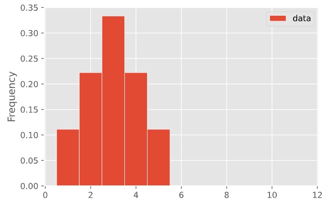
Create a set of data points that has this histogram. (You can do it with a short list of whole numbers.)


What are its mean and median?

In [ ]:
 
In [ ]:
 

Concept Check ✅ – Answer at cc.dsc10.com

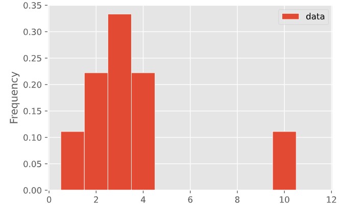
Are the means of these two distributions the same or different? What about the medians?

  • A. Both are the same
  • B. Means are different, medians are same
  • C. Means are same, medians are different
  • D. Both are different

Summary, next time

Summary: Confidence intervals and hypothesis testing

  • Null Hypothesis: The population parameter is equal to some value, $x$.
  • Alternative Hypothesis: The population parameter is not equal to $x$.
  • Cutoff for p-value: p%.
  • Strategy:
    • Construct a (100-p)% confidence interval for the population parameter.
    • If $x$ is not in the interval, we reject the null hypothesis.
    • If $x$ is in the interval, we fail to reject the null hypothesis (since our results are consistent with the null).

Next time

  • What is the standard deviation of a distribution?
  • If we know the mean and standard deviation of a distribution, but nothing else, what can we say about its shape?
  • What is the "normal" distribution, and how does it relate to some of the distributions we've already seen?