The regression line
- The regression line is the line through $(0,0)$ with slope $r$, when both variables are measured in standard units.
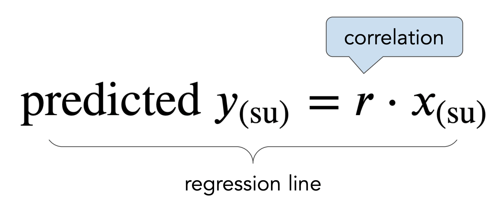
- We use the regression line to make predictions!
# Set up packages for lecture. Don't worry about understanding this code, but
# make sure to run it if you're following along.
import numpy as np
import babypandas as bpd
import pandas as pd
from matplotlib_inline.backend_inline import set_matplotlib_formats
import matplotlib.pyplot as plt
from matplotlib.animation import FuncAnimation, PillowWriter
from scipy import stats
set_matplotlib_formats("svg")
plt.style.use('ggplot')

np.set_printoptions(threshold=20, precision=2, suppress=True)
pd.set_option("display.max_rows", 7)
pd.set_option("display.max_columns", 8)
pd.set_option("display.precision", 2)

# Animations
from IPython.display import display, HTML, IFrame, clear_output
import ipywidgets as widgets

import warnings
warnings.filterwarnings('ignore')

# Demonstration code
def r_scatter(r):
    "Generate a scatter plot with a correlation approximately r"
    x = np.random.normal(0, 1, 1000)
    z = np.random.normal(0, 1, 1000)
    y = r * x + (np.sqrt(1 - r ** 2)) * z
    plt.scatter(x, y)
    plt.xlim(-4, 4)
    plt.ylim(-4, 4)

def show_scatter_grid():
    plt.subplots(1, 4, figsize=(10, 2))
    for i, r in enumerate([-1, -2/3, -1/3, 0]):
        plt.subplot(1, 4, i+1)
        r_scatter(r)
        plt.title(f'r = {np.round(r, 2)}')
    plt.show()
    plt.subplots(1, 4, figsize=(10, 2))
    for i, r in enumerate([1, 2/3, 1/3]):
        plt.subplot(1, 4, i+1)
        r_scatter(r)
        plt.title(f'r = {np.round(r, 2)}')
    plt.subplot(1, 4, 4)
    plt.axis('off')
    plt.show()
Every statistical test and simulation we've run in the second half of the class is related to one of the following four ideas. To solidify your understanding of what we've done, it's a good idea to review past lectures and assignments and see how what we did in each section relates to one of these four ideas.
hybrid = bpd.read_csv('data/hybrid.csv')
hybrid
| vehicle | year | price | acceleration | mpg | class | |
|---|---|---|---|---|---|---|
| 0 | Prius (1st Gen) | 1997 | 24509.74 | 7.46 | 41.26 | Compact |
| 1 | Tino | 2000 | 35354.97 | 8.20 | 54.10 | Compact |
| 2 | Prius (2nd Gen) | 2000 | 26832.25 | 7.97 | 45.23 | Compact |
| ... | ... | ... | ... | ... | ... | ... |
| 150 | C-Max Energi Plug-in | 2013 | 32950.00 | 11.76 | 43.00 | Midsize |
| 151 | Fusion Energi Plug-in | 2013 | 38700.00 | 11.76 | 43.00 | Midsize |
| 152 | Chevrolet Volt | 2013 | 39145.00 | 11.11 | 37.00 | Compact |
153 rows × 6 columns
'acceleration' and 'price'¶Is there an association between these two variables? If so, what kind?
hybrid.plot(kind='scatter', x='acceleration', y='price', figsize=(10, 5));
'mpg' and 'price'¶Is there an association between these two variables? If so, what kind?
hybrid.plot(kind='scatter', x='mpg', y='price', figsize=(10, 5));
Observations:
hybrid.assign(
    km_per_liter=hybrid.get('mpg') * 0.425144,
    yen=hybrid.get('price') * 140.34
).plot(kind='scatter', x='km_per_liter', y='yen', figsize=(10, 5));
def standard_units(any_numbers):
    "Convert any array of numbers to standard units."
    any_numbers = np.array(any_numbers)
    return (any_numbers - any_numbers.mean()) / np.std(any_numbers)
def standardize(df):
    """Return a DataFrame in which all columns of df are converted to standard units."""
    df_su = bpd.DataFrame()
    for column in df.columns:
        df_su = df_su.assign(**{column + ' (su)': standard_units(df.get(column))})
    return df_su
For a given pair of variables:
hybrid_su = standardize(hybrid.get(['price', 'acceleration', 'mpg'])).assign(vehicle=hybrid.get('vehicle'))
hybrid_su
| price (su) | acceleration (su) | mpg (su) | vehicle | |
|---|---|---|---|---|
| 0 | -6.94e-01 | -1.54 | 0.59 | Prius (1st Gen) |
| 1 | -1.86e-01 | -1.28 | 1.76 | Tino |
| 2 | -5.85e-01 | -1.36 | 0.95 | Prius (2nd Gen) |
| ... | ... | ... | ... | ... |
| 150 | -2.98e-01 | -0.07 | 0.75 | C-Max Energi Plug-in |
| 151 | -2.90e-02 | -0.07 | 0.75 | Fusion Energi Plug-in |
| 152 | -8.17e-03 | -0.29 | 0.20 | Chevrolet Volt |
153 rows × 4 columns
'acceleration' and 'price'¶hybrid_su.plot(kind='scatter', x='acceleration (su)', y='price (su)', figsize=(10, 5));
Which cars have 'acceleration's and 'price's that are more than 2 SDs above average?
hybrid_su[(hybrid_su.get('acceleration (su)') > 2) &
          (hybrid_su.get('price (su)') > 2)]
| price (su) | acceleration (su) | mpg (su) | vehicle | |
|---|---|---|---|---|
| 47 | 2.71 | 2.05 | -1.46 | ActiveHybrid X6 |
| 60 | 3.04 | 2.88 | -1.16 | ActiveHybrid 7 |
| 95 | 2.96 | 2.12 | -1.35 | ActiveHybrid 7i |
| 146 | 2.11 | 2.12 | -0.90 | ActiveHybrid 7L |
| 147 | 2.66 | 2.24 | -0.90 | Panamera S |
'mpg' and 'price'¶hybrid_su.plot(kind='scatter', x='mpg (su)', y='price (su)', figsize=(10, 5));
Which cars have close to average 'mpg's and close to average 'price's?
hybrid_su[(hybrid_su.get('mpg (su)') <= 0.3) &
          (hybrid_su.get('mpg (su)') >= -0.3) &
          (hybrid_su.get('price (su)') <= 0.3) &
          (hybrid_su.get('price (su)') >= -0.3)]
| price (su) | acceleration (su) | mpg (su) | vehicle | |
|---|---|---|---|---|
| 10 | -1.24e-01 | -0.56 | -0.26 | Escape |
| 22 | -2.13e-01 | -1.02 | -0.17 | Mercury Mariner |
| 57 | -8.47e-02 | 0.72 | -0.11 | Audi Q5 |
| ... | ... | ... | ... | ... |
| 70 | -2.14e-01 | -0.07 | 0.02 | HS 250h |
| 102 | -2.69e-03 | -0.29 | 0.20 | Chevrolet Volt |
| 152 | -8.17e-03 | -0.29 | 0.20 | Chevrolet Volt |
8 rows × 4 columns
When there is a positive association, most data points fall in the lower left and upper right quadrants.
hybrid_su.plot(kind='scatter', x='acceleration (su)', y='price (su)', figsize=(10, 5))
plt.axvline(0, color='black');
plt.axhline(0, color='black');
When there is a negative association, most data points fall in the upper left and lower right quadrants.
hybrid_su.plot(kind='scatter', x='mpg (su)', y='price (su)', figsize=(10, 5))
plt.axvline(0, color='black');
plt.axhline(0, color='black');
The correlation coefficient $r$ of two variables $x$ and $y$ is defined as the
If x and y are two Series or arrays,
r = (x_su * y_su).mean()
where x_su and y_su are x and y converted to standard units.
Let's calculate $r$ for 'acceleration' and 'price'.
hybrid_su
| price (su) | acceleration (su) | mpg (su) | vehicle | |
|---|---|---|---|---|
| 0 | -6.94e-01 | -1.54 | 0.59 | Prius (1st Gen) |
| 1 | -1.86e-01 | -1.28 | 1.76 | Tino |
| 2 | -5.85e-01 | -1.36 | 0.95 | Prius (2nd Gen) |
| ... | ... | ... | ... | ... |
| 150 | -2.98e-01 | -0.07 | 0.75 | C-Max Energi Plug-in |
| 151 | -2.90e-02 | -0.07 | 0.75 | Fusion Energi Plug-in |
| 152 | -8.17e-03 | -0.29 | 0.20 | Chevrolet Volt |
153 rows × 4 columns
r_acc_price = (hybrid_su.get('acceleration (su)') * hybrid_su.get('price (su)')).mean()
r_acc_price
0.6955778996913982
hybrid_su.plot(kind='scatter', x='acceleration (su)', y='price (su)', figsize=(10, 5))
plt.axvline(0, color='black');
plt.axhline(0, color='black');
Note that the correlation is positive, and most data points fall in the lower left and upper right quadrants!
Let's now calculate $r$ for 'mpg' and 'price'.
hybrid_su
| price (su) | acceleration (su) | mpg (su) | vehicle | |
|---|---|---|---|---|
| 0 | -6.94e-01 | -1.54 | 0.59 | Prius (1st Gen) |
| 1 | -1.86e-01 | -1.28 | 1.76 | Tino |
| 2 | -5.85e-01 | -1.36 | 0.95 | Prius (2nd Gen) |
| ... | ... | ... | ... | ... |
| 150 | -2.98e-01 | -0.07 | 0.75 | C-Max Energi Plug-in |
| 151 | -2.90e-02 | -0.07 | 0.75 | Fusion Energi Plug-in |
| 152 | -8.17e-03 | -0.29 | 0.20 | Chevrolet Volt |
153 rows × 4 columns
r_mpg_price = (hybrid_su.get('mpg (su)') * hybrid_su.get('price (su)')).mean()
r_mpg_price
-0.5318263633683789
hybrid_su.plot(kind='scatter', x='mpg (su)', y='price (su)', figsize=(10, 5));
plt.axvline(0, color='black');
plt.axhline(0, color='black');
Note that the correlation is negative, and most data points fall in the upper left and lower right quadrants!
show_scatter_grid()
Which of the following does the scatter plot below show?
x2 = bpd.DataFrame().assign(
    x=np.arange(-6, 6.1, 0.5),
    y=np.arange(-6, 6.1, 0.5) ** 2
)
x2.plot(kind='scatter', x='x', y='y', figsize=(10, 5));
The data below was collected in the late 1800s by Francis Galton.
galton = bpd.read_csv('data/galton.csv')
galton
| family | father | mother | midparentHeight | children | childNum | gender | childHeight | |
|---|---|---|---|---|---|---|---|---|
| 0 | 1 | 78.5 | 67.0 | 75.43 | 4 | 1 | male | 73.2 |
| 1 | 1 | 78.5 | 67.0 | 75.43 | 4 | 2 | female | 69.2 |
| 2 | 1 | 78.5 | 67.0 | 75.43 | 4 | 3 | female | 69.0 |
| ... | ... | ... | ... | ... | ... | ... | ... | ... |
| 931 | 203 | 62.0 | 66.0 | 66.64 | 3 | 3 | female | 61.0 |
| 932 | 204 | 62.5 | 63.0 | 65.27 | 2 | 1 | male | 66.5 |
| 933 | 204 | 62.5 | 63.0 | 65.27 | 2 | 2 | female | 57.0 |
934 rows × 8 columns
Let's just consider the relationship between mothers' heights and their adult sons' heights.
male_children = galton[galton.get('gender') == 'male']
mom_son = bpd.DataFrame().assign(mom = male_children.get('mother'),
                                 son = male_children.get('childHeight'))
mom_son
| mom | son | |
|---|---|---|
| 0 | 67.0 | 73.2 |
| 4 | 66.5 | 73.5 |
| 5 | 66.5 | 72.5 |
| ... | ... | ... |
| 925 | 60.0 | 66.0 |
| 929 | 66.0 | 64.0 |
| 932 | 63.0 | 66.5 |
481 rows × 2 columns
mom_son.plot(kind='scatter', x='mom', y='son', figsize=(10, 5));
'mom') and her son's height ('son'). 'mom' and 'son'. mom_son_su = standardize(mom_son)
mom_son_su.plot(kind='scatter', x='mom (su)', y='son (su)', figsize=(10, 5));
r_mom_son = (mom_son_su.get('mom (su)') * mom_son_su.get('son (su)')).mean()
r_mom_son
0.32300498368490554
def constant_prediction(prediction):
    mom_son_su.plot(kind='scatter', x='mom (su)', y='son (su)', title=f'Predicting a height of {prediction} SUs for all sons', figsize=(10, 5));
    plt.axhline(prediction, color='orange', lw=4);
    plt.xlim(-3, 3)
    plt.show()

prediction = widgets.FloatSlider(value=-3, min=-3,max=3,step=0.5, description='prediction')
ui = widgets.HBox([prediction])
out = widgets.interactive_output(constant_prediction, {'prediction': prediction})
display(ui, out)
HBox(children=(FloatSlider(value=-3.0, description='prediction', max=3.0, min=-3.0, step=0.5),))
Output()
mom_son_su.plot(kind='scatter', x='mom (su)', y='son (su)', title='A good prediction is the mean height of sons (0 SUs)', figsize=(10, 5));
plt.axhline(0, color='orange', lw=4);
plt.xlim(-3, 3);
def linear_prediction(slope):
    x = np.linspace(-3, 3)
    y = x * slope
    mom_son_su.plot(kind='scatter', x='mom (su)', y='son (su)', figsize=(10, 5));
    plt.plot(x, y, color='orange', lw=4)
    plt.xlim(-3, 3)
    plt.title(r"Predicting sons' heights using $\mathrm{son}_{\mathrm{(su)}}$ = " + str(np.round(slope, 2)) + r"$ \cdot \mathrm{mother}_{\mathrm{(su)}}$")
    plt.show()

slope = widgets.FloatSlider(value=0, min=-1,max=1,step=1/6, description='slope')
ui = widgets.HBox([slope])
out = widgets.interactive_output(linear_prediction, {'slope': slope})
display(ui, out)
HBox(children=(FloatSlider(value=0.0, description='slope', max=1.0, min=-1.0, step=0.16666666666666666),))
Output()
x = np.linspace(-3, 3)
y = x * r_mom_son
mom_son_su.plot(kind='scatter', x='mom (su)', y='son (su)', title=r'A good line goes through the origin and has slope $r$', figsize=(10, 5));
plt.plot(x, y, color='orange', label='regression line', lw=4)
plt.xlim(-3, 3)
plt.legend();
Of course, we'd like to be able to predict a son's height in inches, not just in standard units. Given a mother's height in inches, here's how we'll predict her son's height in inches:
mom_mean = mom_son.get('mom').mean()
mom_sd = np.std(mom_son.get('mom'))
son_mean = mom_son.get('son').mean()
son_sd = np.std(mom_son.get('son'))
def predict_with_r(mom):
    """Return a prediction for the height of a son whose mother has height mom,
    using linear regression.
    """
    mom_su = (mom - mom_mean) / mom_sd
    son_su = r_mom_son * mom_su
    return son_su * son_sd + son_mean
predict_with_r(68)
70.68219686848828
predict_with_r(60)
67.76170758654767
preds = mom_son.assign(
    predicted_height=mom_son.get('mom').apply(predict_with_r)
)
ax = preds.plot(kind='scatter', x='mom', y='son', title='Regression line predictions, in original units', figsize=(10, 5), label='original data')
preds.plot(kind='line', x='mom', y='predicted_height', ax=ax, color='orange', label='regression line', lw=4);
plt.legend();
A course has a midterm (mean 80, standard deviation 15) and a really hard final (mean 50, standard deviation 12).
If the scatter plot comparing midterm & final scores for students looks linearly associated with correlation 0.75, then what is the predicted final exam score for a student who received a 90 on the midterm?
More on regression, including: