# Run this cell to set up packages for lecture.
from lec13_imports import *

Lecture 13 – Distributions and Sampling

DSC 10, Spring 2024

Announcements

• Homework 3 is due tomorrow at 11:59PM.
• The Midterm Project is due on Tuesday, May 7th at 11:59PM.
• Quiz 2 scores are released.
  • Make an appointment with a tutor to review the quiz or prepare for the exam!
• The Midterm Exam is on Friday during your assigned lecture.
  • Everything you need to know about content, format, and logistics is in this Ed post. Post there with any questions.
• In the next class, I'll go over selected problems from last quarter's midterm exam.
  • Read the data description before you arrive, and try some problems if you get a chance.

Agenda

• Probability distributions vs. empirical distributions.
• Populations and samples.
• Parameters and statistics.

🚨 We're moving into the second half of the course, which is more conceptual than the first. Coming to lecture, asking questions, and reading the [textbook] in advance are advised!

Probability distributions vs. empirical distributions

Probability distributions

• Consider a random quantity with various possible values, each of which has some associated probability.

• A probability distribution is a description of:
  • All possible values of the quantity.
  • The theoretical probability of each value.

Example: Probability distribution of a die roll 🎲

The distribution is uniform, meaning that each outcome has the same chance of occurring.

die_faces = np.arange(1, 7, 1)
die = bpd.DataFrame().assign(face=die_faces)
die

	face
0	1
1	2
2	3
3	4
4	5
5	6

bins = np.arange(0.5, 6.6, 1)

# Note that you can add titles to your visualizations, like this!
die.plot(kind='hist', y='face', bins=bins, density=True, ec='w', 
         title='Probability Distribution of a Die Roll',
         figsize=(5, 3))

# You can also set the y-axis label with plt.ylabel.
plt.ylabel('Probability');

Empirical distributions

• Unlike probability distributions, which are theoretical, empirical distributions are based on observations.

• Commonly, these observations are of repetitions of an experiment.

• An empirical distribution describes:
  • All observed values.
  • The proportion of experiments in which each value occurred.

• Unlike probability distributions, empirical distributions represent what actually happened in practice.

Example: Empirical distribution of a die roll 🎲

• Let's simulate a roll by using np.random.choice.
• To simulate the rolling of a die, we must sample with replacement.
  • If we roll a 4, we can roll a 4 again.

num_rolls = 25
many_rolls = np.random.choice(die_faces, num_rolls)
many_rolls

array([5, 1, 5, ..., 1, 1, 3])

(bpd.DataFrame()
 .assign(face=many_rolls) 
 .plot(kind='hist', y='face', bins=bins, density=True, ec='w',
       title=f'Empirical Distribution of {num_rolls} Dice Rolls',
       figsize=(5, 3))
)
plt.ylabel('Probability');

Many die rolls 🎲

What happens as we increase the number of rolls?

for num_rolls in [10, 50, 100, 500, 1000, 5000, 10000]:
    # Don't worry about how .sample works just yet – we'll cover it shortly.
    (die.sample(n=num_rolls, replace=True)
     .plot(kind='hist', y='face', bins=bins, density=True, ec='w', 
           title=f'Distribution of {num_rolls} Die Rolls',
           figsize=(8, 3))
    )

Why does this happen? ⚖️

The law of large numbers states that if a chance experiment is repeated

• many times,
• independently, and
• under the same conditions,

then the proportion of times that an event occurs gets closer and closer to the theoretical probability of that event.

• For example, as you roll a die repeatedly, the proportion of times you roll a 5 gets closer to $\frac{1}{6}$.

• The law of large numbers is why we can use simulations to approximate probability distributions!

Sampling

Populations and samples

• A population is the complete group of people, objects, or events that we want to learn something about.

• It's often infeasible to collect information about every member of a population.

• Instead, we can collect a sample, which is a subset of the population.

• Goal: Estimate the distribution of some numerical variable in the population, using only a sample.
  • For example, suppose we want to know the height of every single UCSD student.
  • It's too hard to collect this information for every single UCSD student – we can't find the population distribution.
  • Instead, we can collect data from a subset of UCSD students, to form a sample distribution.

Sampling strategies

• Question: How do we collect a good sample, so that the sample distribution closely resembles the population distribution?

• Bad idea ❌: Survey whoever you can get ahold of (e.g. internet survey, people in line at Panda Express at PC).
  • Such a sample is known as a convenience sample.
  • Convenience samples often contain hidden sources of bias.

• Good idea ✔️: Select individuals at random.

Simple random sample

A simple random sample (SRS) is a sample drawn uniformly at random without replacement.

• "Uniformly" means every individual has the same chance of being selected.
• "Without replacement" means we won't pick the same individual more than once.

Sampling from a list or array

To perform an SRS from a list or array options, we use np.random.choice(options, n, replace=False).

colleges = np.array(['Revelle', 'John Muir', 'Thurgood Marshall', 
            'Earl Warren', 'Eleanor Roosevelt', 'Sixth', 'Seventh', 'Eighth'])

# Simple random sample of 3 colleges.
np.random.choice(colleges, 3, replace=False)

array(['Eleanor Roosevelt', 'Revelle', 'Seventh'], dtype='<U17')

If we use replace=True, then we're sampling uniformly at random with replacement – there's no simpler term for this.

Example: Distribution of flight delays ✈️

united_full contains information about all United flights leaving SFO between 6/1/15 and 8/31/15.

For this lecture, treat this dataset as our population.

united_full = bpd.read_csv('data/united_summer2015.csv')
united_full

	Date	Flight Number	Destination	Delay
0	6/1/15	73	HNL	257
1	6/1/15	217	EWR	28
2	6/1/15	237	STL	-3
...	...	...	...	...
13822	8/31/15	1994	ORD	3
13823	8/31/15	2000	PHX	-1
13824	8/31/15	2013	EWR	-2

13825 rows × 4 columns

Sampling rows from a DataFrame

If we want to sample rows from a DataFrame, we can use the .sample method on a DataFrame. That is,

df.sample(n)

returns a random subset of n rows of df, drawn without replacement (i.e. the default is replace=False, unlike np.random.choice).

# 5 flights, chosen randomly without replacement.
united_full.sample(5)

	Date	Flight Number	Destination	Delay
3997	6/27/15	1273	OGG	-7
1353	6/10/15	309	IAD	95
9807	8/5/15	329	DEN	-5
6460	7/14/15	718	IAH	0
7127	7/18/15	1531	RDU	-3

# 5 flights, chosen randomly with replacement.
united_full.sample(5, replace=True)

	Date	Flight Number	Destination	Delay
982	6/7/15	1521	SEA	4
346	6/3/15	756	DEN	-9
3264	6/22/15	1683	EWR	17
10126	8/7/15	249	IAD	4
6686	7/15/15	1671	SAN	-6

Note: The probability of seeing the same row multiple times when sampling with replacement is quite low, since our sample size (5) is small relative to the size of the population (13825).

The effect of sample size

• The law of large numbers states that when we repeat a chance experiment more and more times, the empirical distribution will look more and more like the true probability distribution.

• Similarly, if we take a large simple random sample, then the sample distribution is likely to be a good approximation of the true population distribution.

Population distribution of flight delays ✈️

We only need the 'Delay's, so let's select just that column.

united = united_full.get(['Delay'])
united

	Delay
0	257
1	28
2	-3
...	...
13822	3
13823	-1
13824	-2

13825 rows × 1 columns

bins = np.arange(-20, 300, 10)
united.plot(kind='hist', y='Delay', bins=bins, density=True, ec='w', 
            title='Population Distribution of Flight Delays', figsize=(8, 3))
plt.ylabel('Proportion per minute');

Note that this distribution is fixed – nothing about it is random.

Sample distribution of flight delays ✈️

• The 13825 flight delays in united constitute our population.
• Normally, we won't have access to the entire population.
• To replicate a real-world scenario, we will sample from united without replacement.

sample_size = 100 # Change this and see what happens!
(united
 .sample(sample_size)
 .plot(kind='hist', y='Delay', bins=bins, density=True, ec='w',
       title=f'Distribution of Flight Delays in a Sample of Size {sample_size}',
       figsize=(8, 3))
);

Note that as we increase sample_size, the sample distribution of delays looks more and more like the true population distribution of delays.

Parameters and statistics

Terminology

• Statistical inference is the practice of making conclusions about a population, using data from a random sample.

• Parameter: A number associated with the population.
  • Example: The population mean.

• Statistic: A number calculated from the sample.
  • Example: The sample mean.

• A statistic can be used as an estimate for a parameter.

To remember: parameter and population both start with p, statistic and sample both start with s.

Mean flight delay ✈️

Question: What was the average delay of all United flights out of SFO in Summer 2015? 🤔

• We'd love to know the mean delay in the population (parameter), but in practice we'll only have a sample.

• How does the mean delay in the sample (statistic) compare to the mean delay in the population (parameter)?

Population mean

The population mean is a parameter.

# Calculate the mean of the population.
united_mean = united.get('Delay').mean()
united_mean

16.658155515370705

This number (like the population distribution) is fixed, and is not random. In reality, we would not be able to see this number – we can only see it right now because this is a demonstration for teaching!

Sample mean

The sample mean is a statistic. Since it depends on our sample, which was drawn at random, the sample mean is also random.

# Size 100.
united.sample(100).get('Delay').mean()

14.98

• Each time we run the cell above, we are:
  • Collecting a new sample of size 100 from the population, and
  • Computing the sample mean.
• We see a slightly different value on each run of the cell.
  • Sometimes, the sample mean is close to the population mean.
  • Sometimes, it's far away from the population mean.

The effect of sample size

What if we choose a larger sample size?

# Size 1000.
united.sample(1000).get('Delay').mean()

13.865

• Each time we run the above cell, the result is still slightly different.
• However, the results seem to be much closer together – and much closer to the true population mean – than when we used a sample size of 100.
• In general, statistics computed on larger samples tend to be better estimates of population parameters than statistics computed on smaller samples.

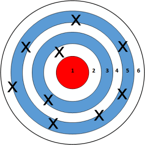
Smaller samples:

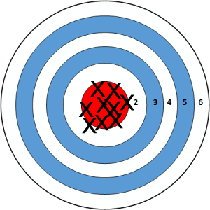
Larger samples:

Probability distribution of a statistic

• The value of a statistic, e.g. the sample mean, is random, because it depends on a random sample.

• Like other random quantities, we can study the "probability distribution" of the statistic (also known as its "sampling distribution").
  • This describes all possible values of the statistic and all the corresponding probabilities.
  • Why? We want to know how different our statistic could have been, had we collected a different sample.

• Unfortunately, this can be hard to calculate exactly.
  • Option 1: Do the math by hand.
  • Option 2: Generate all possible samples and calculate the statistic on each sample.

• So, we'll instead use a simulation to approximate the distribution of the sample statistic.
  • We'll need to generate a lot of possible samples and calculate the statistic on each sample.

Empirical distribution of a statistic

• The empirical distribution of a statistic is based on simulated values of the statistic. It describes:
  • All observed values of the statistic.
  • The proportion of samples in which each value occurred.

• The empirical distribution of a statistic can be a good approximation to the probability distribution of the statistic, if the number of repetitions in the simulation is large.

Distribution of sample means

• To understand how different the sample mean can be in different samples, we'll:
  • Repeatedly draw many samples.
  • Record the mean of each.
  • Draw a histogram of these values.

• The animation below visualizes the process of repeatedly sampling 1000 flights and computing the mean flight delay.

%%capture
anim, anim_means = sampling_animation(united, 1000);

HTML(anim.to_jshtml())

Once Loop Reflect

What's the point?

• In practice, we will only be able to collect one sample and calculate one statistic.
  • Sometimes, that sample will be very representative of the population, and the statistic will be very close to the parameter we are trying to estimate.
  • Other times, that sample will not be as representative of the population, and the statistic will not be very close to the parameter we are trying to estimate.

• The empirical distribution of the sample mean helps us answer the question "what would the sample mean have looked like if we drew a different sample?"

Does sample size matter?

# Sample one thousand flights, two thousand times.
sample_size = 1000
repetitions = 2000
sample_means = np.array([])

for n in np.arange(repetitions):
    m = united.sample(sample_size).get('Delay').mean()
    sample_means = np.append(sample_means, m)

bpd.DataFrame().assign(sample_means=sample_means) \
               .plot(kind='hist', bins=np.arange(10, 25, 0.5), density=True, ec='w',
                     title=f'Distribution of Sample Mean with Sample Size {sample_size}',
                     figsize=(10, 5));
    
plt.axvline(x=united_mean, c='black', linewidth=4, label='population mean')
plt.legend();

Concept Check ✅ – Answer at cc.dsc10.com

We just sampled one thousand flights, two thousand times. If we now sample one hundred flights, two thousand times, how will the histogram change?

• A. Narrower
• B. Wider
• C. Shifted left
• D. Shifted right
• E. Unchanged

How we sample matters!

• So far, we've taken large simple random samples from the full population.
  • Simple random samples are taken without replacement.
  • If the population is large enough, then it doesn't really matter if we sample with or without replacement.

• The sample mean, for samples like this, is a good approximation of the population mean.

• But this is not always the case if we sample differently.

Summary, coming soon

Summary

• The probability distribution of a random quantity describes the values it takes on along with the probability of each value occurring.
• An empirical distribution describes the values and frequencies of the results of a random experiment.
  • With more trials of an experiment, the empirical distribution gets closer to the probability distribution.
• A population distribution describes the values and frequencies of some characteristic of a population.
• A sample distribution describes the values and frequencies of some characteristic of a sample, which is a subset of a population.
  • When we take a simple random sample, as we increase our sample size, the sample distribution gets closer and closer to the population distribution.
• A parameter is a number associated with a population, and a statistic is a number associated with a sample.
• We can use statistics calculated on a random samples to estimate population parameters.
  • For example, to estimate the mean of a population, we can calculate the mean of the sample.
  • Larger samples tend to lead to better estimates.

Coming soon

• Large random samples lead to better estimates, but how do we balance this with the practical challenges associated with collecting a very large sample?
• Soon we'll introduce a clever solution called bootstrapping 🥾, which allows us to leverage the power of a single sample to get good estimates!