# Run this cell, which imports packages and sets up some formatting to make lectures display nicely.
from lec04_imports import *
Announcements
- Lab 1 is due Saturday at 11:59PM.
- Submit early and avoid submission errors.
- Quiz 1 is coming up on Monday in discussion section.
- This will be a 20 minute paper-based quiz consisting of short answer and multiple choice questions.
- Afterwards, the TA can help with Homework 1 questions.
- The quiz covers Lectures 1 through 4, or BPD 1-9 in the
babypandasnotes.- Review both of these materials to study.
- Do last week's extra practice problems and attend the extra practice session this Friday!
- No aids are allowed (no notes, no calculators, no computers, no reference sheet). Questions are designed with this in mind.
- This will be a 20 minute paper-based quiz consisting of short answer and multiple choice questions.
- Come to office hours (see the schedule here) and post on Ed for help!
Agenda
- Arrays.
- Ranges.
- DataFrames.
Note:
- Remember to check the resources tab of the course website for programming resources.
- Some key links moving forward:
Arrays
Recap: arrays
- Arrays are provided by a module called
numpythat we need to import to use.
import numpy as np
- Arrays store sequences of values of the same data type.
- To create an array, we pass a list as input to the
np.arrayfunction.
temperature_array = np.array([68, 73, 70, 74, 76, 72, 74])
temperature_array
array([68, 73, 70, 74, 76, 72, 74])
- Use square brackets with the position number to access an array element. The first element is in position 0.
temperature_array
array([68, 73, 70, 74, 76, 72, 74])
temperature_array[1]
73
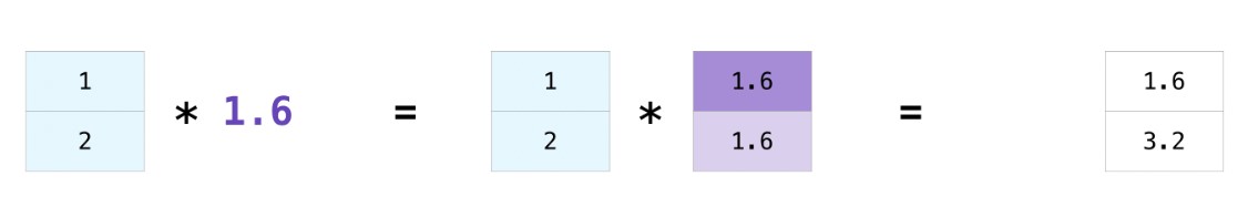
Array-number arithmetic
Arrays make it easy to perform the same operation to every element. This behavior is formally known as "broadcasting".
temperature_array
array([68, 73, 70, 74, 76, 72, 74])
# Convert all temperatures to Celsius.
(5 / 9) * (temperature_array - 32)
array([20. , 22.78, 21.11, 23.33, 24.44, 22.22, 23.33])
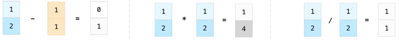
Element-wise arithmetic
- We can apply arithmetic operations to multiple arrays, provided they have the same length.
- The result is computed element-wise, which means that the arithmetic operation is applied to one pair of elements from each array at a time.
a = np.array([4, 5, -1])
b = np.array([2, 3, 2])
a ** 2 + b ** 2
array([20, 34, 5])
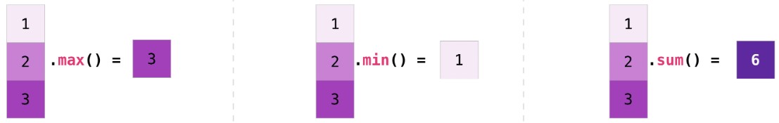
Array methods
Arrays work with a variety of methods, which are functions designed to operate specifically on arrays.
Call these methods using dot notation, e.g.
array_name.method().
temperature_array.max()
76
temperature_array.mean()
72.42857142857143
Example: TikTok views 🎬
We decided to make a Series of TikToks called "A Day in the Life of a Baby Panda". The number of views we've received on these videos are stored in the array views below.
views = np.array([158, 352, 195, 1423916, 46])
Some questions:
- What is the difference between each video's view count and the average view count?
views - views.mean()
array([-284775.4, -284581.4, -284738.4, 1138982.6, -284887.4])
- How many views above average did our most viewed video receive?
(views - views.mean()).max()
1138982.6
- It has been estimated that TikTok pays their creators \$0.03 per 1000 views. If this is true, how many dollars did we earn on our most viewed video? 💸
views.max() * 0.03 / 1000
42.717479999999995
Ranges
Motivation
We often find ourselves needing to make arrays like this:
day_of_month = np.array([
    1, 2, 3, 4, 5, 6, 7, 8, 9, 10, 11, 12,
    13, 14, 15, 16, 17, 18, 19, 20, 21, 22,
    23, 24, 25, 26, 27, 28, 29, 30, 31
])
There needs to be an easier way to do this!
Ranges
- A range is an array of evenly spaced numbers. We create ranges using
np.arange. - The most general way to create a range is
np.arange(start, end, step). This returns an array such that:- The first number is
start. By default,startis 0. - All subsequent numbers are spaced out by
step, until (but excluding)end. By default,stepis 1.
- The first number is
# Start at 0, end before 8, step by 1.
# This will be our most common use-case!
np.arange(8)
array([0, 1, 2, 3, 4, 5, 6, 7])
# Start at 5, end before 10, step by 1.
np.arange(5, 10)
array([5, 6, 7, 8, 9])
# Start at 3, end before 32, step by 5.
np.arange(3, 32, 5)
array([ 3, 8, 13, 18, 23, 28])
Extra practice
The step size in np.arange can be fractional, or even negative. Predict what arrays will be produced by each line of code below. Then copy each line into a code cell and run it to see if you're right.
np.arange(-3, 2, 0.5)

np.arange(1, -10, -3)
...
Ellipsis
...
Ellipsis
Challenge
🎉 Congrats! 🎉 You won the lottery 💰. Here's how your payout works: on the first day of September, you are paid \$0.01. Every day thereafter, your pay doubles, so on the second day you're paid \$0.02, on the third day you're paid \$0.04, on the fourth day you're paid \$0.08, and so on.
September has 30 days.
Write a one-line expression that uses the numbers 2 and 30, along with the function np.arange and the method .sum(), that computes the total amount in dollars you will be paid in September.
...
Ellipsis
After trying the challenge problem on your own, watch this walkthrough 🎥 video.
DataFrames
pandas
pandasis a Python package that allows us to work with tabular data – that is, data in the form of a table that we might otherwise work with as a spreadsheet (in Excel or Google Sheets).pandasis the tool for doing data science in Python.

But pandas is not so cute...

Enter babypandas!
- We at UCSD have created a smaller, nicer version of
pandascalledbabypandas. - It keeps the important stuff and has much better error messages.
- It's easier to learn, but is still valid
pandascode. You are learningpandas!- Think of it like learning how to build LEGOs with many, but not all, of the possible Lego blocks. You're still learning how to build LEGOs, and you can still build cool things!

DataFrames in babypandas 🐼
- Tables in
babypandas(andpandas) are called "DataFrames." - To use DataFrames, we'll need to import
babypandas.
import babypandas as bpd
Reading data from a file 📖
We'll usually work with data stored in the CSV format. CSV stands for "comma-separated values."
We can read in a CSV using
bpd.read_csv(...). Replace the...with a path to the CSV file relative to your notebook; if the file is in the same folder as your notebook, this is just the name of the file.
# Our CSV file is stored not in the same folder as our notebook,
# but within a folder called data.
states = bpd.read_csv('data/states.csv')
states
| State | Region | Capital City | Population | Land Area | Party | |
|---|---|---|---|---|---|---|
| 0 | Alabama | South | Montgomery | 5024279 | 50645 | Republican |
| 1 | Alaska | West | Juneau | 733391 | 570641 | Republican |
| 2 | Arizona | West | Phoenix | 7151502 | 113594 | Republican |
| 3 | Arkansas | South | Little Rock | 3011524 | 52035 | Republican |
| 4 | California | West | Sacramento | 39538223 | 155779 | Democratic |
| ... | ... | ... | ... | ... | ... | ... |
| 45 | Virginia | South | Richmond | 8631393 | 39490 | Democratic |
| 46 | Washington | West | Olympia | 7705281 | 66456 | Democratic |
| 47 | West Virginia | South | Charleston | 1793716 | 24038 | Republican |
| 48 | Wisconsin | Midwest | Madison | 5893718 | 54158 | Republican |
| 49 | Wyoming | West | Cheyenne | 576851 | 97093 | Republican |
50 rows × 6 columns
About the data 🗽
Most of the data is self-explanatory, but there are a few things to note:
'Population'figures come from the 2020 census.
'Land Area'is measured in square miles.
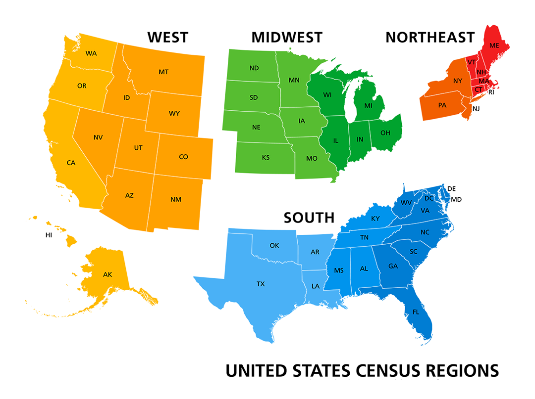
- The
'Region'column places each state in one of four regions, as determined by the US Census Bureau.
- The
'Party'column classifies each state as'Democratic'or'Republican'based on a political science measurement called the Cook Partisan Voter Index.
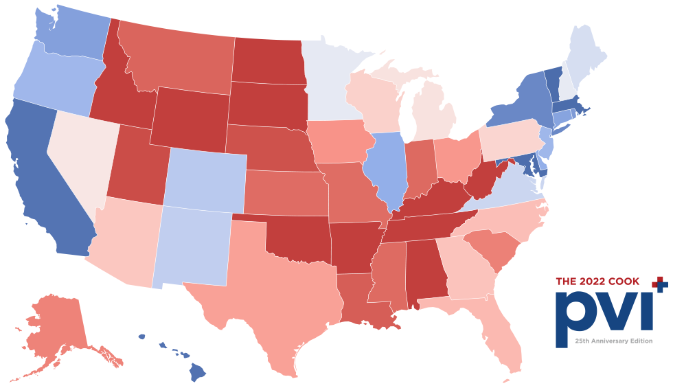 (source)
Structure of a DataFrame
- DataFrames have columns and rows.
- Think of each column as an array. Columns contain data of the same type.
- Each column has a label, e.g.
'Capital City'and'Land Area'.- Column labels are stored as strings.
- Each row has a label too – these are shown in bold at the start of the row.
- Right now, the row labels are 0, 1, 2, and so on.
- Together, the row labels are called the index. The index is not a column!
# This DataFrame has 50 rows and 6 columns.
states
| State | Region | Capital City | Population | Land Area | Party | |
|---|---|---|---|---|---|---|
| 0 | Alabama | South | Montgomery | 5024279 | 50645 | Republican |
| 1 | Alaska | West | Juneau | 733391 | 570641 | Republican |
| 2 | Arizona | West | Phoenix | 7151502 | 113594 | Republican |
| 3 | Arkansas | South | Little Rock | 3011524 | 52035 | Republican |
| 4 | California | West | Sacramento | 39538223 | 155779 | Democratic |
| ... | ... | ... | ... | ... | ... | ... |
| 45 | Virginia | South | Richmond | 8631393 | 39490 | Democratic |
| 46 | Washington | West | Olympia | 7705281 | 66456 | Democratic |
| 47 | West Virginia | South | Charleston | 1793716 | 24038 | Republican |
| 48 | Wisconsin | Midwest | Madison | 5893718 | 54158 | Republican |
| 49 | Wyoming | West | Cheyenne | 576851 | 97093 | Republican |
50 rows × 6 columns
Example 1: Population density
Key concepts: Accessing columns, performing calculations with them, and adding new columns.
Finding population density
Question: What is the population density of each state, in people per square mile?
states
| State | Region | Capital City | Population | Land Area | Party | |
|---|---|---|---|---|---|---|
| 0 | Alabama | South | Montgomery | 5024279 | 50645 | Republican |
| 1 | Alaska | West | Juneau | 733391 | 570641 | Republican |
| 2 | Arizona | West | Phoenix | 7151502 | 113594 | Republican |
| 3 | Arkansas | South | Little Rock | 3011524 | 52035 | Republican |
| 4 | California | West | Sacramento | 39538223 | 155779 | Democratic |
| ... | ... | ... | ... | ... | ... | ... |
| 45 | Virginia | South | Richmond | 8631393 | 39490 | Democratic |
| 46 | Washington | West | Olympia | 7705281 | 66456 | Democratic |
| 47 | West Virginia | South | Charleston | 1793716 | 24038 | Republican |
| 48 | Wisconsin | Midwest | Madison | 5893718 | 54158 | Republican |
| 49 | Wyoming | West | Cheyenne | 576851 | 97093 | Republican |
50 rows × 6 columns
- We have, separately, the population and land area of each state.
- Steps:
- Get the
'Population'column. - Get the
'Land Area'column. - Divide these columns element-wise.
- Add a new column to the DataFrame with these results.
- Get the
Step 1 – Getting the 'Population' column
- We can get a column from a DataFrame using
.get(column_name). - 🚨 Column names are case sensitive!
- Column names are strings, so we need to use quotes.
- The result looks like a 1-column DataFrame, but is actually a Series.
states
| State | Region | Capital City | Population | Land Area | Party | |
|---|---|---|---|---|---|---|
| 0 | Alabama | South | Montgomery | 5024279 | 50645 | Republican |
| 1 | Alaska | West | Juneau | 733391 | 570641 | Republican |
| 2 | Arizona | West | Phoenix | 7151502 | 113594 | Republican |
| 3 | Arkansas | South | Little Rock | 3011524 | 52035 | Republican |
| 4 | California | West | Sacramento | 39538223 | 155779 | Democratic |
| ... | ... | ... | ... | ... | ... | ... |
| 45 | Virginia | South | Richmond | 8631393 | 39490 | Democratic |
| 46 | Washington | West | Olympia | 7705281 | 66456 | Democratic |
| 47 | West Virginia | South | Charleston | 1793716 | 24038 | Republican |
| 48 | Wisconsin | Midwest | Madison | 5893718 | 54158 | Republican |
| 49 | Wyoming | West | Cheyenne | 576851 | 97093 | Republican |
50 rows × 6 columns
states.get('Population')
0      5024279
1       733391
2      7151502
3      3011524
4     39538223
        ...
45     8631393
46     7705281
47     1793716
48     5893718
49      576851
Name: Population, Length: 50, dtype: int64
Digression: Series
- A Series is like an array, but with an index.
- In particular, Series support arithmetic, just like arrays.
states.get('Population')
0      5024279
1       733391
2      7151502
3      3011524
4     39538223
        ...
45     8631393
46     7705281
47     1793716
48     5893718
49      576851
Name: Population, Length: 50, dtype: int64
type(states.get('Population'))
babypandas.bpd.Series
Steps 2 and 3 – Getting the 'Land Area' column and dividing element-wise
states.get('Land Area')
0      50645
1     570641
2     113594
3      52035
4     155779
       ...
45     39490
46     66456
47     24038
48     54158
49     97093
Name: Land Area, Length: 50, dtype: int64
- Just like with arrays, we can perform arithmetic operations with two Series, as long as they have the same length and same index.
- Operations happen element-wise (by matching up corresponding index values), and the result is also a Series.
states.get('Population') / states.get('Land Area')
0      99.21
1       1.29
2      62.96
3      57.87
4     253.81
       ...
45    218.57
46    115.95
47     74.62
48    108.82
49      5.94
Length: 50, dtype: float64
Step 4 – Adding the densities to the DataFrame as a new column
- Use
.assign(name_of_column=data_in_series)to assign a Series (or array, or list) to a DataFrame. - 🚨 Don't put quotes around
name_of_column. - This creates a new DataFrame, which we must save to a variable if we want to keep using it.
states.assign(
    Density=states.get('Population') / states.get('Land Area')
)
| State | Region | Capital City | Population | Land Area | Party | Density | |
|---|---|---|---|---|---|---|---|
| 0 | Alabama | South | Montgomery | 5024279 | 50645 | Republican | 99.21 |
| 1 | Alaska | West | Juneau | 733391 | 570641 | Republican | 1.29 |
| 2 | Arizona | West | Phoenix | 7151502 | 113594 | Republican | 62.96 |
| 3 | Arkansas | South | Little Rock | 3011524 | 52035 | Republican | 57.87 |
| 4 | California | West | Sacramento | 39538223 | 155779 | Democratic | 253.81 |
| ... | ... | ... | ... | ... | ... | ... | ... |
| 45 | Virginia | South | Richmond | 8631393 | 39490 | Democratic | 218.57 |
| 46 | Washington | West | Olympia | 7705281 | 66456 | Democratic | 115.95 |
| 47 | West Virginia | South | Charleston | 1793716 | 24038 | Republican | 74.62 |
| 48 | Wisconsin | Midwest | Madison | 5893718 | 54158 | Republican | 108.82 |
| 49 | Wyoming | West | Cheyenne | 576851 | 97093 | Republican | 5.94 |
50 rows × 7 columns
states
| State | Region | Capital City | Population | Land Area | Party | |
|---|---|---|---|---|---|---|
| 0 | Alabama | South | Montgomery | 5024279 | 50645 | Republican |
| 1 | Alaska | West | Juneau | 733391 | 570641 | Republican |
| 2 | Arizona | West | Phoenix | 7151502 | 113594 | Republican |
| 3 | Arkansas | South | Little Rock | 3011524 | 52035 | Republican |
| 4 | California | West | Sacramento | 39538223 | 155779 | Democratic |
| ... | ... | ... | ... | ... | ... | ... |
| 45 | Virginia | South | Richmond | 8631393 | 39490 | Democratic |
| 46 | Washington | West | Olympia | 7705281 | 66456 | Democratic |
| 47 | West Virginia | South | Charleston | 1793716 | 24038 | Republican |
| 48 | Wisconsin | Midwest | Madison | 5893718 | 54158 | Republican |
| 49 | Wyoming | West | Cheyenne | 576851 | 97093 | Republican |
50 rows × 6 columns
states = states.assign(
    Density=states.get('Population') / states.get('Land Area')
)
states
| State | Region | Capital City | Population | Land Area | Party | Density | |
|---|---|---|---|---|---|---|---|
| 0 | Alabama | South | Montgomery | 5024279 | 50645 | Republican | 99.21 |
| 1 | Alaska | West | Juneau | 733391 | 570641 | Republican | 1.29 |
| 2 | Arizona | West | Phoenix | 7151502 | 113594 | Republican | 62.96 |
| 3 | Arkansas | South | Little Rock | 3011524 | 52035 | Republican | 57.87 |
| 4 | California | West | Sacramento | 39538223 | 155779 | Democratic | 253.81 |
| ... | ... | ... | ... | ... | ... | ... | ... |
| 45 | Virginia | South | Richmond | 8631393 | 39490 | Democratic | 218.57 |
| 46 | Washington | West | Olympia | 7705281 | 66456 | Democratic | 115.95 |
| 47 | West Virginia | South | Charleston | 1793716 | 24038 | Republican | 74.62 |
| 48 | Wisconsin | Midwest | Madison | 5893718 | 54158 | Republican | 108.82 |
| 49 | Wyoming | West | Cheyenne | 576851 | 97093 | Republican | 5.94 |
50 rows × 7 columns
Example 2: Exploring population density
Key concept: Computing statistics of columns using Series methods.
Questions
- What is the highest population density of any one state?
- What is the average population density across all states?
Series, like arrays, have helpful methods, including .min(), .max(), and .mean().
states.get('Density').max()
1263.1212945335872
What state does this correspond to? We'll see how to find out shortly!
Other statistics:
states.get('Density').min()
1.2852055845969708
states.get('Density').mean()
206.54513507096468
states.get('Density').median()
108.31649013462203
# Lots of information at once!
states.get('Density').describe()
count      50.00
mean      206.55
std       274.93
min         1.29
25%        47.06
50%       108.32
75%       224.57
max      1263.12
Name: Density, dtype: float64
Example 3: Which state has the highest population density?
Key concepts: Sorting. Accessing using integer positions.
Step 1 – Sorting the DataFrame
- Use the
.sort_values(by=column_name)method to sort.- The
by=can be omitted, but helps with readability.
- The
- Like most DataFrame methods, this returns a new DataFrame.
states.sort_values(by='Density')
| State | Region | Capital City | Population | Land Area | Party | Density | |
|---|---|---|---|---|---|---|---|
| 1 | Alaska | West | Juneau | 733391 | 570641 | Republican | 1.29 |
| 49 | Wyoming | West | Cheyenne | 576851 | 97093 | Republican | 5.94 |
| 25 | Montana | West | Helena | 1084225 | 145546 | Republican | 7.45 |
| 33 | North Dakota | Midwest | Bismarck | 779094 | 69001 | Republican | 11.29 |
| 40 | South Dakota | Midwest | Pierre | 886667 | 75811 | Republican | 11.70 |
| ... | ... | ... | ... | ... | ... | ... | ... |
| 19 | Maryland | South | Annapolis | 6177224 | 9707 | Democratic | 636.37 |
| 6 | Connecticut | Northeast | Hartford | 3605944 | 4842 | Democratic | 744.72 |
| 20 | Massachusetts | Northeast | Boston | 7029917 | 7800 | Democratic | 901.27 |
| 38 | Rhode Island | Northeast | Providence | 1097379 | 1034 | Democratic | 1061.29 |
| 29 | New Jersey | Northeast | Trenton | 9288994 | 7354 | Democratic | 1263.12 |
50 rows × 7 columns
This sorts, but in ascending order (small to large). The opposite would be nice!
Step 1 – Sorting the DataFrame in descending order
- Use
.sort_values(by=column_name, ascending=False)to sort in descending order. ascendingis an optional argument. If omitted, it will be set toTrueby default.- This is an example of a keyword argument, or a named argument.
- If we want to specify the sorting order, we must use the keyword
ascending=.
ordered_states = states.sort_values(by='Density', ascending=False)
ordered_states
| State | Region | Capital City | Population | Land Area | Party | Density | |
|---|---|---|---|---|---|---|---|
| 29 | New Jersey | Northeast | Trenton | 9288994 | 7354 | Democratic | 1263.12 |
| 38 | Rhode Island | Northeast | Providence | 1097379 | 1034 | Democratic | 1061.29 |
| 20 | Massachusetts | Northeast | Boston | 7029917 | 7800 | Democratic | 901.27 |
| 6 | Connecticut | Northeast | Hartford | 3605944 | 4842 | Democratic | 744.72 |
| 19 | Maryland | South | Annapolis | 6177224 | 9707 | Democratic | 636.37 |
| ... | ... | ... | ... | ... | ... | ... | ... |
| 40 | South Dakota | Midwest | Pierre | 886667 | 75811 | Republican | 11.70 |
| 33 | North Dakota | Midwest | Bismarck | 779094 | 69001 | Republican | 11.29 |
| 25 | Montana | West | Helena | 1084225 | 145546 | Republican | 7.45 |
| 49 | Wyoming | West | Cheyenne | 576851 | 97093 | Republican | 5.94 |
| 1 | Alaska | West | Juneau | 733391 | 570641 | Republican | 1.29 |
50 rows × 7 columns
# We must specify the role of False by using ascending=,
# otherwise Python does not know how to interpret this.
states.sort_values(by='Density', False)
Step 2 – Extracting the state name
- We saw that the most densely populated state is New Jersey, but how do we extract that information using code?
- First, grab an entire column as a Series.
- Navigate to a particular entry of the Series using
.iloc[integer_position].ilocstands for "integer location" and is used to count the rows, starting at 0.
ordered_states
| State | Region | Capital City | Population | Land Area | Party | Density | |
|---|---|---|---|---|---|---|---|
| 29 | New Jersey | Northeast | Trenton | 9288994 | 7354 | Democratic | 1263.12 |
| 38 | Rhode Island | Northeast | Providence | 1097379 | 1034 | Democratic | 1061.29 |
| 20 | Massachusetts | Northeast | Boston | 7029917 | 7800 | Democratic | 901.27 |
| 6 | Connecticut | Northeast | Hartford | 3605944 | 4842 | Democratic | 744.72 |
| 19 | Maryland | South | Annapolis | 6177224 | 9707 | Democratic | 636.37 |
| ... | ... | ... | ... | ... | ... | ... | ... |
| 40 | South Dakota | Midwest | Pierre | 886667 | 75811 | Republican | 11.70 |
| 33 | North Dakota | Midwest | Bismarck | 779094 | 69001 | Republican | 11.29 |
| 25 | Montana | West | Helena | 1084225 | 145546 | Republican | 7.45 |
| 49 | Wyoming | West | Cheyenne | 576851 | 97093 | Republican | 5.94 |
| 1 | Alaska | West | Juneau | 733391 | 570641 | Republican | 1.29 |
50 rows × 7 columns
ordered_states.get('State')
29       New Jersey
38     Rhode Island
20    Massachusetts
6       Connecticut
19         Maryland
          ...
40     South Dakota
33     North Dakota
25          Montana
49          Wyoming
1            Alaska
Name: State, Length: 50, dtype: object
# We want the first entry of the Series, which is at "integer location" 0.
ordered_states.get('State').iloc[0]
'New Jersey'
- The row label that goes with New Jersey is 29, because our original data was alphabetized by state and New Jersey is the 30th state alphabetically. But we don't use the row label when accessing with
iloc; we use the integer position counting from the top.
- If we try to use the row label (29) with
iloc, we get the state with the 30th highest population density, which is not New Jersey.
ordered_states.get('State').iloc[29]
'Minnesota'
Example 4: What is the population density of Pennsylvania?
Key concept: Accessing using row labels.
Population density of Pennsylvania
We know how to get the 'Density' of all states. How do we find the one that corresponds to Pennsylvania?
states
| State | Region | Capital City | Population | Land Area | Party | Density | |
|---|---|---|---|---|---|---|---|
| 0 | Alabama | South | Montgomery | 5024279 | 50645 | Republican | 99.21 |
| 1 | Alaska | West | Juneau | 733391 | 570641 | Republican | 1.29 |
| 2 | Arizona | West | Phoenix | 7151502 | 113594 | Republican | 62.96 |
| 3 | Arkansas | South | Little Rock | 3011524 | 52035 | Republican | 57.87 |
| 4 | California | West | Sacramento | 39538223 | 155779 | Democratic | 253.81 |
| ... | ... | ... | ... | ... | ... | ... | ... |
| 45 | Virginia | South | Richmond | 8631393 | 39490 | Democratic | 218.57 |
| 46 | Washington | West | Olympia | 7705281 | 66456 | Democratic | 115.95 |
| 47 | West Virginia | South | Charleston | 1793716 | 24038 | Republican | 74.62 |
| 48 | Wisconsin | Midwest | Madison | 5893718 | 54158 | Republican | 108.82 |
| 49 | Wyoming | West | Cheyenne | 576851 | 97093 | Republican | 5.94 |
50 rows × 7 columns
# Which one is Pennsylvania?
states.get('Density')
0      99.21
1       1.29
2      62.96
3      57.87
4     253.81
       ...
45    218.57
46    115.95
47     74.62
48    108.82
49      5.94
Name: Density, Length: 50, dtype: float64
Utilizing the index
- When we load in a DataFrame from a CSV, columns have meaningful names, but rows do not.
bpd.read_csv('data/states.csv')
| State | Region | Capital City | Population | Land Area | Party | |
|---|---|---|---|---|---|---|
| 0 | Alabama | South | Montgomery | 5024279 | 50645 | Republican |
| 1 | Alaska | West | Juneau | 733391 | 570641 | Republican |
| 2 | Arizona | West | Phoenix | 7151502 | 113594 | Republican |
| 3 | Arkansas | South | Little Rock | 3011524 | 52035 | Republican |
| 4 | California | West | Sacramento | 39538223 | 155779 | Democratic |
| ... | ... | ... | ... | ... | ... | ... |
| 45 | Virginia | South | Richmond | 8631393 | 39490 | Democratic |
| 46 | Washington | West | Olympia | 7705281 | 66456 | Democratic |
| 47 | West Virginia | South | Charleston | 1793716 | 24038 | Republican |
| 48 | Wisconsin | Midwest | Madison | 5893718 | 54158 | Republican |
| 49 | Wyoming | West | Cheyenne | 576851 | 97093 | Republican |
50 rows × 6 columns
- The row labels (or the index) are how we refer to specific rows. Instead of using numbers, let's refer to these rows by the names of the states they correspond to.
- This way, we can easily identify, for example, which row corresponds to Pennsylvania.
Setting the index
- To change the index, use
.set_index(column_name). - Row labels should be unique identifiers.
- Each row should have a different, descriptive name that corresponds to the contents of that row's data.
states
| State | Region | Capital City | Population | Land Area | Party | Density | |
|---|---|---|---|---|---|---|---|
| 0 | Alabama | South | Montgomery | 5024279 | 50645 | Republican | 99.21 |
| 1 | Alaska | West | Juneau | 733391 | 570641 | Republican | 1.29 |
| 2 | Arizona | West | Phoenix | 7151502 | 113594 | Republican | 62.96 |
| 3 | Arkansas | South | Little Rock | 3011524 | 52035 | Republican | 57.87 |
| 4 | California | West | Sacramento | 39538223 | 155779 | Democratic | 253.81 |
| ... | ... | ... | ... | ... | ... | ... | ... |
| 45 | Virginia | South | Richmond | 8631393 | 39490 | Democratic | 218.57 |
| 46 | Washington | West | Olympia | 7705281 | 66456 | Democratic | 115.95 |
| 47 | West Virginia | South | Charleston | 1793716 | 24038 | Republican | 74.62 |
| 48 | Wisconsin | Midwest | Madison | 5893718 | 54158 | Republican | 108.82 |
| 49 | Wyoming | West | Cheyenne | 576851 | 97093 | Republican | 5.94 |
50 rows × 7 columns
states.set_index('State')
| Region | Capital City | Population | Land Area | Party | Density | |
|---|---|---|---|---|---|---|
| State | ||||||
| Alabama | South | Montgomery | 5024279 | 50645 | Republican | 99.21 |
| Alaska | West | Juneau | 733391 | 570641 | Republican | 1.29 |
| Arizona | West | Phoenix | 7151502 | 113594 | Republican | 62.96 |
| Arkansas | South | Little Rock | 3011524 | 52035 | Republican | 57.87 |
| California | West | Sacramento | 39538223 | 155779 | Democratic | 253.81 |
| ... | ... | ... | ... | ... | ... | ... |
| Virginia | South | Richmond | 8631393 | 39490 | Democratic | 218.57 |
| Washington | West | Olympia | 7705281 | 66456 | Democratic | 115.95 |
| West Virginia | South | Charleston | 1793716 | 24038 | Republican | 74.62 |
| Wisconsin | Midwest | Madison | 5893718 | 54158 | Republican | 108.82 |
| Wyoming | West | Cheyenne | 576851 | 97093 | Republican | 5.94 |
50 rows × 6 columns
- Now there is one fewer column. When you set the index, a column becomes the index, and the old index disappears.
- 🚨 Like most DataFrame methods,
.set_indexreturns a new DataFrame; it does not modify the original DataFrame.
states
| State | Region | Capital City | Population | Land Area | Party | Density | |
|---|---|---|---|---|---|---|---|
| 0 | Alabama | South | Montgomery | 5024279 | 50645 | Republican | 99.21 |
| 1 | Alaska | West | Juneau | 733391 | 570641 | Republican | 1.29 |
| 2 | Arizona | West | Phoenix | 7151502 | 113594 | Republican | 62.96 |
| 3 | Arkansas | South | Little Rock | 3011524 | 52035 | Republican | 57.87 |
| 4 | California | West | Sacramento | 39538223 | 155779 | Democratic | 253.81 |
| ... | ... | ... | ... | ... | ... | ... | ... |
| 45 | Virginia | South | Richmond | 8631393 | 39490 | Democratic | 218.57 |
| 46 | Washington | West | Olympia | 7705281 | 66456 | Democratic | 115.95 |
| 47 | West Virginia | South | Charleston | 1793716 | 24038 | Republican | 74.62 |
| 48 | Wisconsin | Midwest | Madison | 5893718 | 54158 | Republican | 108.82 |
| 49 | Wyoming | West | Cheyenne | 576851 | 97093 | Republican | 5.94 |
50 rows × 7 columns
states = states.set_index('State')
states
| Region | Capital City | Population | Land Area | Party | Density | |
|---|---|---|---|---|---|---|
| State | ||||||
| Alabama | South | Montgomery | 5024279 | 50645 | Republican | 99.21 |
| Alaska | West | Juneau | 733391 | 570641 | Republican | 1.29 |
| Arizona | West | Phoenix | 7151502 | 113594 | Republican | 62.96 |
| Arkansas | South | Little Rock | 3011524 | 52035 | Republican | 57.87 |
| California | West | Sacramento | 39538223 | 155779 | Democratic | 253.81 |
| ... | ... | ... | ... | ... | ... | ... |
| Virginia | South | Richmond | 8631393 | 39490 | Democratic | 218.57 |
| Washington | West | Olympia | 7705281 | 66456 | Democratic | 115.95 |
| West Virginia | South | Charleston | 1793716 | 24038 | Republican | 74.62 |
| Wisconsin | Midwest | Madison | 5893718 | 54158 | Republican | 108.82 |
| Wyoming | West | Cheyenne | 576851 | 97093 | Republican | 5.94 |
50 rows × 6 columns
# Which one is Pennsylvania? The one whose row label is "Pennsylvania"!
states.get('Density')
State
Alabama           99.21
Alaska             1.29
Arizona           62.96
Arkansas          57.87
California       253.81
                  ...
Virginia         218.57
Washington       115.95
West Virginia     74.62
Wisconsin        108.82
Wyoming            5.94
Name: Density, Length: 50, dtype: float64
Accessing using the row label
To pull out one particular entry of a DataFrame corresponding to a row and column with certain labels:
- Use
.get(column_name)to extract the entire column as a Series. - Use
.loc[]to access the element of a Series with a particular row label.
In this class, we'll always first access a column, then a row (but row, then column is also possible).
states.get('Density')
State
Alabama           99.21
Alaska             1.29
Arizona           62.96
Arkansas          57.87
California       253.81
                  ...
Virginia         218.57
Washington       115.95
West Virginia     74.62
Wisconsin        108.82
Wyoming            5.94
Name: Density, Length: 50, dtype: float64
states.get('Density').loc['Pennsylvania']
290.60858681804973
Summary: Accessing elements of a DataFrame
- First,
.getthe appropriate column as a Series. - Then, use one of two ways to access an element of a Series:
.iloc[]uses the integer position..loc[]uses the row label.- Each is best for different scenarios.
states.get('Density')
State
Alabama           99.21
Alaska             1.29
Arizona           62.96
Arkansas          57.87
California       253.81
                  ...
Virginia         218.57
Washington       115.95
West Virginia     74.62
Wisconsin        108.82
Wyoming            5.94
Name: Density, Length: 50, dtype: float64
states.get('Density').iloc[4]
253.80971119342146
states.get('Density').loc['California']
253.80971119342146
Note
- Sometimes the integer position and row label are the same.
- This happens by default with
bpd.read_csv.
bpd.read_csv('data/states.csv')
| State | Region | Capital City | Population | Land Area | Party | |
|---|---|---|---|---|---|---|
| 0 | Alabama | South | Montgomery | 5024279 | 50645 | Republican |
| 1 | Alaska | West | Juneau | 733391 | 570641 | Republican |
| 2 | Arizona | West | Phoenix | 7151502 | 113594 | Republican |
| 3 | Arkansas | South | Little Rock | 3011524 | 52035 | Republican |
| 4 | California | West | Sacramento | 39538223 | 155779 | Democratic |
| ... | ... | ... | ... | ... | ... | ... |
| 45 | Virginia | South | Richmond | 8631393 | 39490 | Democratic |
| 46 | Washington | West | Olympia | 7705281 | 66456 | Democratic |
| 47 | West Virginia | South | Charleston | 1793716 | 24038 | Republican |
| 48 | Wisconsin | Midwest | Madison | 5893718 | 54158 | Republican |
| 49 | Wyoming | West | Cheyenne | 576851 | 97093 | Republican |
50 rows × 6 columns
bpd.read_csv('data/states.csv').get('Capital City').loc[35]
'Oklahoma City'
bpd.read_csv('data/states.csv').get('Capital City').iloc[35]
'Oklahoma City'
Summary, next time
Summary
- Arrays make it easy to perform arithmetic operations on all elements of an array and to perform element-wise operations on multiple arrays.
- Ranges are arrays of equally-spaced numbers.
- We learned many DataFrame methods and techniques. Don't feel the need to memorize them all right away.
- Instead, refer to this lecture, the DSC 10 reference sheet, the
babypandasnotes, and thebabypandasdocumentation when working on assignments. - Over time, these techniques will become more and more familiar. Lab 1 will walk you through many of them.
- Practice! Frame your own questions using this dataset and try to answer them.
Next time
We'll frame more questions and learn more DataFrame manipulation techniques to answer them. In particular, we'll learn about querying and grouping.