import pandas as pd
import numpy as np

import matplotlib.pyplot as plt
plt.rcParams['figure.figsize'] = (10, 5)

import util

Lecture 1 – Introduction, Data Science Lifecycle

DSC 80, Spring 2022

Welcome to DSC 80! 🎉

Agenda

• Who are we?
• What does a data scientist do?
• What is this course about, and how will it run?
• The data science lifecycle.

About the instructor

Suraj Rampure (call me Suraj, pronounced “soo-rudge”)

• Originally from Windsor, ON, Canada 🇨🇦.
• BS (’20) and MS (’21) in EECS from UC Berkeley 🐻.
  • Designed and taught several data science courses as a student there.
• Third quarter teaching at UCSD 🌴, and first time teaching DSC 80.
  • Also teaching DSC 90 (History of Data Science) this quarter.
  • Previously taught DSC 10 (x2) and DSC 40A.
• Outside the classroom 👨‍🏫: watching basketball, traveling, eating, watching TikTok, FaceTiming my dog 🐶, etc.

Me with my mom, my dog, and my friend over spring break.

Course staff

In addition to the instructor, we have several other course staff members who are here to support you in discussion, office hours, and Campuswire.

• 1 graduate TA: Murali Dandu.
• 11 undergraduate tutors: Nicole Brye, Aven Huang, Shubham Kaushal, Karthikeya Manchala, Yash Potdar, Costin Smiliovici, Anjana Sriram, Ruojia Tao, Du Xiang, Sheng Yang, and Winston Yu.

Learn more about them at dsc80.com/staff.

What is data science? 🤔

What is data science?

Everyone seems to have their own definition of what data science is.

The DSC 10 definition

In DSC 10, we told you that science is about drawing useful conclusions from data using computation.

• Exploration.
  • Identifying patterns in information.
  • Uses visualizations.
• Prediction.
  • Making informed guesses.
  • Uses machine learning and optimization.
• Inference.
  • Quantifying whether those predictions are reliable.
  • Uses randomization.

Let's look at some other definitions.

What is data science?

In 2010, Drew Conway published his famous Data Science Venn Diagram.

What is data science?

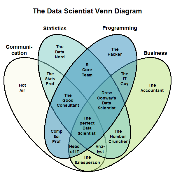
There isn't agreement on which "Venn Diagram" is correct!

• Why not? The field is new and rapidly developing.
• Make sure you're solid on the fundamentals, then find a niche that you enjoy.
• Read Kolassa, Battle of the Data Science Venn Diagrams.

What does a data scientist do?

In 2016, O'Reilly administered a Data Scientice Salary Survey. Part of the survey asked self-identified data scientists what tasks they do on a regular basis.

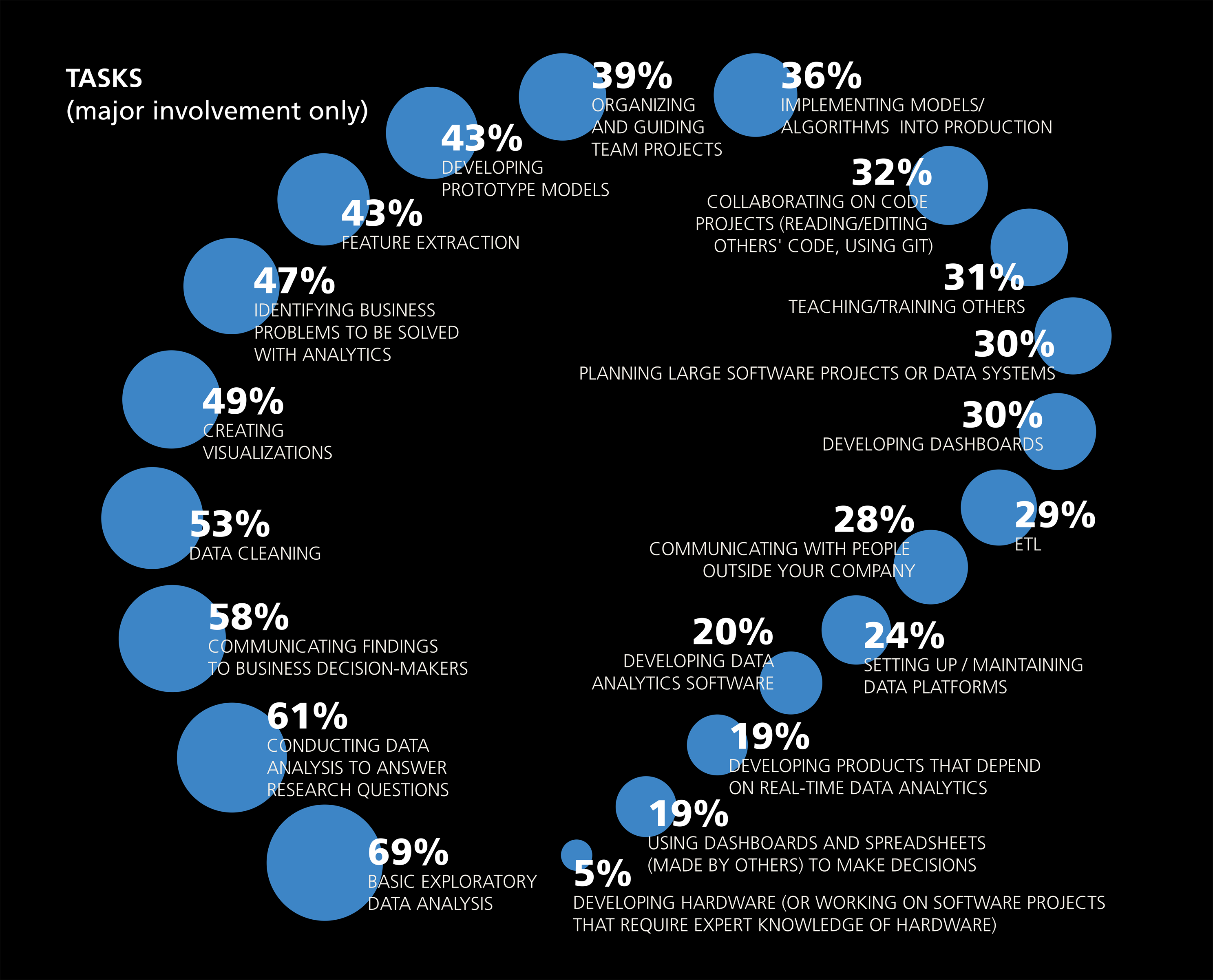
What do you notice?

What does a data scientist do?

My take: in DSC 80, and in the DSC major more broadly, we are equipping you to ask and answer questions using data.

Let's look at some examples of data science in practice.

Analyzing Wordle trends

Moving average of the average number of guesses taken for each Wordle word, based on patterns shared on Twitter. (source)

Analyzing Wordle trends

Number of Wordle patterns shared per day on Twitter. (source)

Forecasting COVID cases

Results of the UCSD_NEU-DeepGLEAM COVID cases forecasting model for the upcoming week (source).

Forecasting COVID cases

Evaluation of case forecasts showed that more reported cases than expected fell outside the forecast prediction intervals for extended periods of time. Given this low reliability, COVID-19 case forecasts will no longer be posted by the Centers for Disease Control and Prevention. - CDC.gov

Depixelizer

A "Face Depixelizer" released in 2020 takes pixelated images and generates images that are perceptually realistic and downscale correctly.

What happened here? Why do you think this happened?

Data science involves people 🧍

The decisions that we make as data scientists have the potential to impact the livelihoods of other people.

• COVID case forecasting.
• Admissions and hiring.
• Hyper-personalized ad recommendations.
• Criminal sentencing.

Warning! ⚠️

• Good data analysis is not:

  • A simple application of a statistics formula.
  • A simple application of statistical software.

• There are many tools out there for data science, but they are merely tools. They don’t do any of the important thinking – that's where you come in!

“The purpose of computing is insight, not numbers.” - R. Hamming. Numerical Methods for Scientists and Engineers (1962).

Course content

Course goals

In this course, you will...

• Practice translating potentially vague questions into quantitative questions about measurable observations.
• Learn to reason about 'black-box' processes (e.g. complicated models).
• Understand computational and statistical implications of working with data.
• Learn to use real data tools (e.g. love the documentation!).
• Get a taste of the "life of a data scientist".

Course outcomes

After this course, you will...

• Be prepared for internships and data science "take home" interviews!
• Be ready to create your own portfolio of personal projects.
• Have the background and maturity to succeed in the upper-division.

Topics

This course was desgined by a former data scientist at Amazon (Aaron Fraenkel). As such, you'll be learning skills that you need to know as a data scientist.

• Week 1: DataFrames in pandas
• Week 2: Messy Data and Hypothesis Testing
• Week 3: Combining Data
• Week 4: Permutation Testing and Missing Values
• Week 5: Imputation, Midterm Exam
• Week 6: Web Scraping and Regex
• Week 7: Feature Engineering
• Week 8: Modeling in scikit-learn
• Week 9: Model Evaluation
• Week 10: Review, Final Exam

Course logistics

Course website

The course website is your one-stop-shop for all things related to the course.

dsc80.com

Make sure to read the syllabus!

Getting set up

• Campuswire: Q&A forum. Must be active here, since this is where all announcements will be made. You should have been added already; if not, join here (code 2756).
• Gradescope: Where you will submit all assignments for autograding, and where all of your grades will live. You should have been added already; contact us if not.

In addition, you must also fill out our Welcome + Alternate Exams Form.

Accessing course content on GitHub

You will access all course content by pulling the course GitHub repository:

github.com/dsc-courses/dsc80-2022-sp

We will post HTML versions of lecture notebooks on the course website, but otherwise you must pull from this repository to access all course materials (including blank copies of assignments).

Environment setup

• You have two choices:
  • Set up your own Python environment (strongly recommended).
  • Use DataHub.
• Either way, follow the instructions on the Tech Support page of the course website.
• Once you set up your environment, you will pull the course repo every time a new assignment comes out.
• Note: You will submit your work to Gradescope directly, without using Git.
• Will post a demo video with Lab 1.

Course meetings

• Lectures are MWF 3-3:50PM or 4-4:50PM. Come in-person at Center Hall 109 or via Zoom. Anyone can attend either section.
• Discussions are W 6-6:50PM or 7-7:50PM. Come in-person at Pepper Canyon Hall 122 or via Zoom. Anyone can attend either section.

Assignments

In this course, you will learn by doing!

• Labs (25%): 9 total. Due weekly on Mondays, starting next week.
• Projects (30%): 5 total. Usually due on Thursdays, and usually have a "checkpoint."
• Discussions (2% EC): 8 total. Extra credit.

In DSC 80, assignments will usually consist of both a Jupyter Notebook and a .py file. You will write your code in the .py file; the Jupyter Notebook will contain problem descriptions and test cases. Lab 1 will explain the workflow.

Exams

• Midterm Exam (15%): Wednesday, April 27th during your assigned lecture slot (3-3:50PM or 4-4:50PM). In-person in Center 109.
• Final Exam (25%): Saturday, June 4th from 11:30AM-2:30PM. In-person, location TBD.
• Fill out the Welcome + Alternate Exams Form to tell us if you have a conflict.

Resources

• Your main resource will be lecture notebooks.
• Most lectures also have supplemental readings that come from our course notes, notes.dsc80.com.
• Other resources:
  • Wes McKinney. "Python for Data Analysis".
  • DSC 10 Course Notes – great refresher on babypandas.
  • Principles and Techniques of Data Science.
  • Computational and Inferential Thinking.
  • pandastutor.com.
  • As the quarter progresses, we'll add more resources to the Resources tab of the course website.

Support 🫂

It is no secret that this course requires a lot of work - becoming fluent with working with data is hard!

• You will learn how to solve problems independently – documentation and the internet will be your friends.
• Learning how to effectively check your work and debug is extremely useful.

Once you've tried to solve problems on your own, we're glad to help.

• Office hours are offered both remotely and in-person. See the Calendar 📆 for details.
• Campuswire is your friend too. Make your conceptual questions public, and make your debugging questions private.

The data science lifecycle 🚴

The scientific method

You learned about the scientific method in elementary school.

However, it hides a lot of complexity.

• Where did the hypothesis come from?
• What data are you modeling? Is the data sufficient?
• Under which conditions are the conclusions valid?

The data science lifecycle

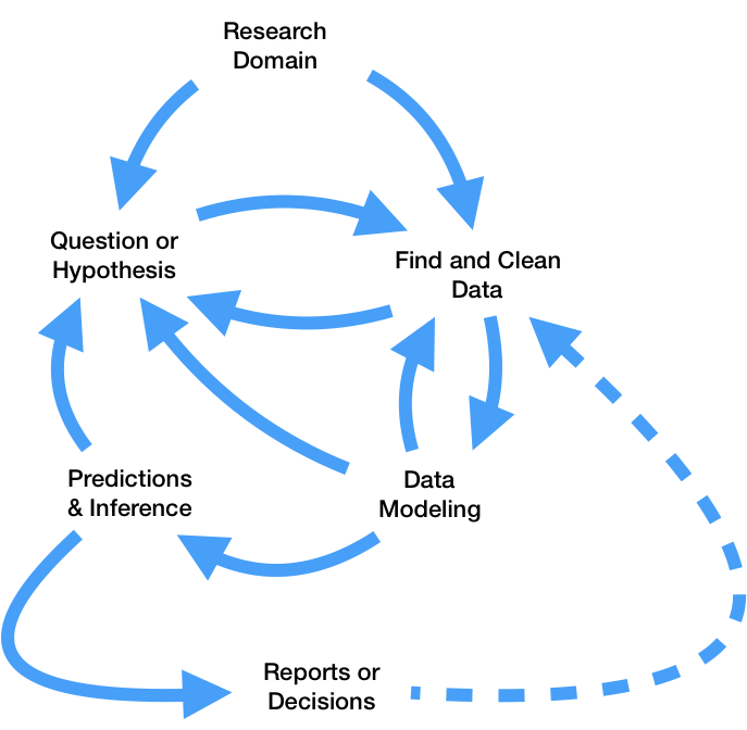
All steps lead to more questions!

Example: San Diego employee salaries

Research Domain and Questions

We have our domain – City of San Diego employee salaries. What are some questions we might want to ask?

• Which jobs have the highest and lowest salaries?
• Who works part-time? full-time?
• Are salaries "fair"?
• What is the predicted 2025 salary for the mayor of San Diego?
• Can we build a "profile" of the average San Diego city employee?

Context

Why is this dataset relevant?

• Journalists might search for salary anomalies.
• Auditors may want actionable advice on fair employment practices.

Find and Clean Data

Initial look at the data

• Transparent California publishes the salaries of all City of San Diego employees.
• The latest available data is from 2020.

salary_path = util.safe_download('https://transcal.s3.amazonaws.com/public/export/san-diego-2020.csv')

salaries = pd.read_csv(salary_path)
util.anonymize_names(salaries)
salaries

	Employee Name	Job Title	Base Pay	Overtime Pay	Other Pay	Benefits	Total Pay	Total Pay & Benefits	Year	Notes	Agency	Status
0	Michael Xxxx	Police Officer	117691.0	187290.0	13331.00	36380.0	318312.0	354692.0	2020	NaN	San Diego	FT
1	Gary Xxxx	Police Officer	117691.0	160062.0	42946.00	31795.0	320699.0	352494.0	2020	NaN	San Diego	FT
2	Eric Xxxx	Fire Engineer	35698.0	204462.0	69121.00	38362.0	309281.0	347643.0	2020	NaN	San Diego	PT
3	Gregg Xxxx	Retirement Administrator	305000.0	0.0	12814.00	24792.0	317814.0	342606.0	2020	NaN	San Diego	FT
4	Joseph Xxxx	Fire Battalion Chief	94451.0	157778.0	48151.00	42096.0	300380.0	342476.0	2020	NaN	San Diego	FT
...	...	...	...	...	...	...	...	...	...	...	...	...
12600	Elena Xxxx	Asst Eng-Civil	0.0	2.0	0.00	0.0	2.0	2.0	2020	NaN	San Diego	PT
12601	Gary Xxxx	Police Officer	0.0	2.0	0.00	0.0	2.0	2.0	2020	NaN	San Diego	PT
12602	Sara Xxxx	Asst Planner	0.0	1.0	0.00	0.0	1.0	1.0	2020	NaN	San Diego	PT
12603	Kevin Xxxx	Project Ofcr 1	0.0	1.0	0.00	0.0	1.0	1.0	2020	NaN	San Diego	PT
12604	Deedrick Xxxx	Utility Worker 2	0.0	0.0	1.00	0.0	1.0	1.0	2020	NaN	San Diego	PT

12605 rows × 12 columns

Aside on privacy and ethics

• Employee names correspond to real people.
• Be careful when dealing with PII (personably identifiable information).
  • Only work with the data that is needed for your analysis.
  • Even when data is public, people have a reasonable right to privacy.

Data cleaning

• As we saw in the O'Reilly's survey results either, data cleaning is a huge component of real-world data science.
  • You didn't get much exposure to it in DSC 10, but you will in DSC 80.
• Let's look at summary statistics for each of our numeric columns.
  • Do you notice anything strange?
  • What are the implications on data reliability?

# .T is for transpose()
salaries.describe().T

	count	mean	std	min	25%	50%	75%	max
Base Pay	12605.0	56066.707180	35773.864476	0.0	32714.0	54725.0	77512.0	305000.0
Overtime Pay	12605.0	8789.100198	18507.729611	-293.0	0.0	588.0	9174.0	204462.0
Benefits	12605.0	15456.868068	11183.968318	-39.0	6425.0	14549.0	22745.0	86066.0
Total Pay	12605.0	75181.321618	49634.174460	0.0	41177.0	71354.0	106903.0	320699.0
Total Pay & Benefits	12605.0	90638.189687	58833.565854	1.0	52478.0	86226.0	128147.0	354692.0
Year	12605.0	2020.000000	0.000000	2020.0	2020.0	2020.0	2020.0	2020.0
Notes	0.0	NaN	NaN	NaN	NaN	NaN	NaN	NaN

• Someone had an 'Overtime Pay' of -\$293!
• The 'Other Pay' column contained numbers, why doesn't it appear here?
• How many people have salaries of \$0?
• Why is there a 'Notes' column that is missing for everybody?

Empirical distribution of salaries

Let's plot the distribution of salaries.

salaries['Total Pay'].plot(kind='hist', density=True, bins=50, ec='w', 
                           title='City of San Diego Employee Salaries');

Discussion Question

Which of the following best describe the distribution of San Diego employee salaries?

• A. Right-skewed, unimodal
• B. Right-skewed, bimodal
• C. Left-skewed, unimodal
• D. Left-skewed, bimodal

🙋 To answer, go to yellkey.com/job.

Empirical distribution of salaries

Let's draw the distribution of salaries separately for part-time and full-time employees.

bystatus = salaries.groupby('Status')
bystatus['Total Pay'].plot(kind='kde', title='City of San Diego Employee Salaries, Part-Time vs. Full-Time')
plt.legend(bystatus.groups);

Question: Does gender influence pay?

• Do employees of different genders have similar pay?
• The salary dataset we downloaded does not contain employee gender, so we can't answer this question using just the data we have.

salaries.head()

	Employee Name	Job Title	Base Pay	Overtime Pay	Other Pay	Benefits	Total Pay	Total Pay & Benefits	Year	Notes	Agency	Status
0	Michael Xxxx	Police Officer	117691.0	187290.0	13331.00	36380.0	318312.0	354692.0	2020	NaN	San Diego	FT
1	Gary Xxxx	Police Officer	117691.0	160062.0	42946.00	31795.0	320699.0	352494.0	2020	NaN	San Diego	FT
2	Eric Xxxx	Fire Engineer	35698.0	204462.0	69121.00	38362.0	309281.0	347643.0	2020	NaN	San Diego	PT
3	Gregg Xxxx	Retirement Administrator	305000.0	0.0	12814.00	24792.0	317814.0	342606.0	2020	NaN	San Diego	FT
4	Joseph Xxxx	Fire Battalion Chief	94451.0	157778.0	48151.00	42096.0	300380.0	342476.0	2020	NaN	San Diego	FT

• We do, however, have the first name of each employee.

Social Security Administration baby names 👶

• The US Social Security Administration (SSA) keeps track of the first name, birth year, and assigned gender at birth for all babies born in the US.
• We can somehow combine the SSA's dataset with the salaries dataset to infer the gender of San Diego employees.

names_path = util.safe_download('https://www.ssa.gov/oact/babynames/names.zip')

import pathlib

dfs = []
for path in pathlib.Path('data/names/').glob('*.txt'):
    year = int(str(path)[14:18])
    if year >= 1964:
        df = pd.read_csv(path, names=['firstname', 'gender', 'count']).assign(year=year)
        dfs.append(df)
        
names = pd.concat(dfs)
names

	firstname	gender	count	year
0	Emily	F	25957	2000
1	Hannah	F	23084	2000
2	Madison	F	19968	2000
3	Ashley	F	17997	2000
4	Sarah	F	17706	2000
...	...	...	...	...
32025	Zyheem	M	5	2019
32026	Zykel	M	5	2019
32027	Zyking	M	5	2019
32028	Zyn	M	5	2019
32029	Zyran	M	5	2019

1399746 rows × 4 columns

We began compiling the baby name list in 1997, with names dating back to 1880. At the time of a child’s birth, parents supply the name to us when applying for a child’s Social Security card, thus making Social Security America’s source for the most popular baby names. Please share this with your friends and family—and help us spread the word on social media. - Social Security’s Top Baby Names for 2020

Exploring names

• The only values of 'gender' in names are 'M' and 'F'.
• Many names have non-zero counts for both 'M' and 'F'.
• Most names occur only a few times per year, but a few names occur very often.

names.head()

	firstname	gender	count	year
0	Emily	F	25957	2000
1	Hannah	F	23084	2000
2	Madison	F	19968	2000
3	Ashley	F	17997	2000
4	Sarah	F	17706	2000

# Get the count of each unique value in the 'gender' column
names['gender'].value_counts()

F    838442
M    561304
Name: gender, dtype: int64

# Look at a single name
names[names['firstname'] == 'Billy']

	firstname	gender	count	year
10875	Billy	F	8	2000
18042	Billy	M	670	2000
14851	Billy	F	6	2014
20007	Billy	M	287	2014
19912	Billy	M	281	2015
...	...	...	...	...
18364	Billy	M	208	2020
21031	Billy	M	458	2008
14044	Billy	F	6	2018
18949	Billy	M	262	2018
18836	Billy	M	245	2019

104 rows × 4 columns

# Look at various summary statistics
names.describe()

	count	year
count	1.399746e+06	1.399746e+06
mean	1.459451e+02	1.996861e+03
std	1.194298e+03	1.542586e+01
min	5.000000e+00	1.964000e+03
25%	7.000000e+00	1.985000e+03
50%	1.100000e+01	1.999000e+03
75%	3.000000e+01	2.010000e+03
max	8.529100e+04	2.020000e+03

Data Modeling

Determining the most common gender for each name

• Recall, our goal is to infer the gender of each San Diego city employee. To do this, we need a mapping of first names to genders.

• A (very imperfect) model: If someone has a name that is predominantly used by gender $g$, we'll infer their gender to be $g$.

• Approach: Create a DataFrame indexed by 'firstname' that describes the total number of 'F' and 'M' babies in names for each unique 'firstname'.
  • If there are more female babies born with a given name than male babies, we will "classify" the name as female.
  • Otherwise, we will classify the name as male.

Determining the most common gender for each name

counts_by_gender = (
    names
    .groupby(['firstname', 'gender'])
    .sum()
    .reset_index()
    .pivot('firstname', 'gender', 'count')
    .fillna(0)
)
counts_by_gender

gender	F	M
firstname
Aaban	0.0	120.0
Aabha	46.0	0.0
Aabid	0.0	16.0
Aabidah	5.0	0.0
Aabir	0.0	10.0
...	...	...
Zyvion	0.0	5.0
Zyvon	0.0	7.0
Zyyanna	6.0	0.0
Zyyon	0.0	6.0
Zzyzx	0.0	10.0

91360 rows × 2 columns

counts_by_gender['F'] > counts_by_gender['M']

firstname
Aaban      False
Aabha       True
Aabid      False
Aabidah     True
Aabir      False
           ...  
Zyvion     False
Zyvon      False
Zyyanna     True
Zyyon      False
Zzyzx      False
Length: 91360, dtype: bool

genders = counts_by_gender.assign(gender=np.where(counts_by_gender['F'] > counts_by_gender['M'], 'F', 'M'))
genders

gender	F	M	gender
firstname
Aaban	0.0	120.0	M
Aabha	46.0	0.0	F
Aabid	0.0	16.0	M
Aabidah	5.0	0.0	F
Aabir	0.0	10.0	M
...	...	...	...
Zyvion	0.0	5.0	M
Zyvon	0.0	7.0	M
Zyyanna	6.0	0.0	F
Zyyon	0.0	6.0	M
Zzyzx	0.0	10.0	M

91360 rows × 3 columns

Adding a 'gender' column to salaries

This involves two steps:

1. Extracting just the first name from 'Employee Name'.
2. Merging salaries and genders.

# Add firstname column
salaries['firstname'] = salaries['Employee Name'].str.split().str[0]
salaries

	Employee Name	Job Title	Base Pay	Overtime Pay	Other Pay	Benefits	Total Pay	Total Pay & Benefits	Year	Notes	Agency	Status	firstname
0	Michael Xxxx	Police Officer	117691.0	187290.0	13331.00	36380.0	318312.0	354692.0	2020	NaN	San Diego	FT	Michael
1	Gary Xxxx	Police Officer	117691.0	160062.0	42946.00	31795.0	320699.0	352494.0	2020	NaN	San Diego	FT	Gary
2	Eric Xxxx	Fire Engineer	35698.0	204462.0	69121.00	38362.0	309281.0	347643.0	2020	NaN	San Diego	PT	Eric
3	Gregg Xxxx	Retirement Administrator	305000.0	0.0	12814.00	24792.0	317814.0	342606.0	2020	NaN	San Diego	FT	Gregg
4	Joseph Xxxx	Fire Battalion Chief	94451.0	157778.0	48151.00	42096.0	300380.0	342476.0	2020	NaN	San Diego	FT	Joseph
...	...	...	...	...	...	...	...	...	...	...	...	...	...
12600	Elena Xxxx	Asst Eng-Civil	0.0	2.0	0.00	0.0	2.0	2.0	2020	NaN	San Diego	PT	Elena
12601	Gary Xxxx	Police Officer	0.0	2.0	0.00	0.0	2.0	2.0	2020	NaN	San Diego	PT	Gary
12602	Sara Xxxx	Asst Planner	0.0	1.0	0.00	0.0	1.0	1.0	2020	NaN	San Diego	PT	Sara
12603	Kevin Xxxx	Project Ofcr 1	0.0	1.0	0.00	0.0	1.0	1.0	2020	NaN	San Diego	PT	Kevin
12604	Deedrick Xxxx	Utility Worker 2	0.0	0.0	1.00	0.0	1.0	1.0	2020	NaN	San Diego	PT	Deedrick

12605 rows × 13 columns

# Merge salaries and genders
salaries_with_gender = salaries.merge(genders[['gender']], on='firstname', how='left')
salaries_with_gender

	Employee Name	Job Title	Base Pay	Overtime Pay	Other Pay	Benefits	Total Pay	Total Pay & Benefits	Year	Notes	Agency	Status	firstname	gender
0	Michael Xxxx	Police Officer	117691.0	187290.0	13331.00	36380.0	318312.0	354692.0	2020	NaN	San Diego	FT	Michael	M
1	Gary Xxxx	Police Officer	117691.0	160062.0	42946.00	31795.0	320699.0	352494.0	2020	NaN	San Diego	FT	Gary	M
2	Eric Xxxx	Fire Engineer	35698.0	204462.0	69121.00	38362.0	309281.0	347643.0	2020	NaN	San Diego	PT	Eric	M
3	Gregg Xxxx	Retirement Administrator	305000.0	0.0	12814.00	24792.0	317814.0	342606.0	2020	NaN	San Diego	FT	Gregg	M
4	Joseph Xxxx	Fire Battalion Chief	94451.0	157778.0	48151.00	42096.0	300380.0	342476.0	2020	NaN	San Diego	FT	Joseph	M
...	...	...	...	...	...	...	...	...	...	...	...	...	...	...
12600	Elena Xxxx	Asst Eng-Civil	0.0	2.0	0.00	0.0	2.0	2.0	2020	NaN	San Diego	PT	Elena	F
12601	Gary Xxxx	Police Officer	0.0	2.0	0.00	0.0	2.0	2.0	2020	NaN	San Diego	PT	Gary	M
12602	Sara Xxxx	Asst Planner	0.0	1.0	0.00	0.0	1.0	1.0	2020	NaN	San Diego	PT	Sara	F
12603	Kevin Xxxx	Project Ofcr 1	0.0	1.0	0.00	0.0	1.0	1.0	2020	NaN	San Diego	PT	Kevin	M
12604	Deedrick Xxxx	Utility Worker 2	0.0	0.0	1.00	0.0	1.0	1.0	2020	NaN	San Diego	PT	Deedrick	M

12605 rows × 14 columns

Predictions and Inference

Question: Does gender influence pay?

This was our original question. Let's find out!

pd.concat([
    salaries_with_gender.groupby('gender')['Total Pay'].describe().T,
    salaries_with_gender['Total Pay'].describe().rename('All')
], axis=1)

	F	M	All
count	4075.000000	8043.000000	12605.000000
mean	63865.752883	81297.593808	75181.321618
std	43497.853002	51567.740425	49634.174460
min	1.000000	0.000000	0.000000
25%	33084.000000	44900.000000	41177.000000
50%	59975.000000	77579.000000	71354.000000
75%	89854.000000	117374.500000	106903.000000
max	295904.000000	320699.000000	320699.000000

• Unfortunately, there's a fairly large difference between the mean salaries of male employees and female employees.
• A similar difference also exists for the median.
• Can this difference be explained by random chance?

A hypothesis test

• Null Hypothesis: Gender is independent of salary, and any observed differences are due to random chance.
• Alternate Hypothesis: Gender is not independent of salary. Female employees earn less than male employees.

n_female = np.count_nonzero(salaries_with_gender['gender'] == 'F')
n_female

4075

Strategy:

• Randomly select 4075 employees from salaries_with_gender and compute their median salary.
• Repeat this many times.
• See where the observed median salary of female employees lies in this empirical distribution.

Running the hypothesis test

# Observed statistic
female_median = salaries_with_gender.loc[salaries_with_gender['gender'] == 'F']['Total Pay'].median()

# Simulate 1000 samples of size n_female from the population
medians = np.array([])
for _ in np.arange(1000):
    median = salaries_with_gender.sample(n_female)['Total Pay'].median()
    medians = np.append(medians, median)

medians[:10]

array([72263., 69699., 70880., 70554., 71104., 72511., 70781., 70781.,
       72096., 70755.])

title='Median salary of randomly chosen groups from population'
pd.Series(medians).plot(kind='hist', density=True, ec='w', title=title);
plt.axvline(x=female_median, color='red')
plt.legend(['Observed Median Salary of Female Employees', 'Median Salaries of Random Groups']);

• Our hypothesis test has a p-value of 0, so we reject the null.
  • Under the assumption that gender is independent of salary, the chance of seeing a median salary this low is essentially 0.

Next time

• While performing this analysis, we made several assumptions. What were they, and how did they affect our results?
• After wrapping up this example, we'll dive deep into pandas!
• Lab 1 will be released tomorrow!