import pandas as pd
import numpy as np

import matplotlib.pyplot as plt
plt.rcParams['figure.figsize'] = (10, 5)

import util

Lecture 2 – Pandas 🐼

DSC 80, Spring 2022

Announcements

• Lab 1 is due on Monday, April 4th at 11:59PM.
  • Watch this video 🎥 for setup instructions.
• Discussion 1 is today from 7-7:50PM or 8-8:50PM (in-person in PCNYH 122 or remote via Zoom).
  • There was a typo in the discussion times stated in Lecture 1.
  • Remember that discussion assignments can be submitted for extra credit!
• Don't forget to fill out the Welcome + Alternate Exams Form by Monday as well.

Agenda

• Wrap up our case study of City of San Diego employee salaries.
• Introduction to pandas.
  • DataFrames, Series, and Indexes.
• Selecting rows and columns using [] and loc.

The data science lifecycle

Recap: City of San Diego salary data

Our dataset is downloaded from Transparent California.

salary_path = util.safe_download('https://transcal.s3.amazonaws.com/public/export/san-diego-2020.csv')

salaries = pd.read_csv(salary_path)
util.anonymize_names(salaries)
salaries

	Employee Name	Job Title	Base Pay	Overtime Pay	Other Pay	Benefits	Total Pay	Total Pay & Benefits	Year	Notes	Agency	Status
0	Michael Xxxx	Police Officer	117691.0	187290.0	13331.00	36380.0	318312.0	354692.0	2020	NaN	San Diego	FT
1	Gary Xxxx	Police Officer	117691.0	160062.0	42946.00	31795.0	320699.0	352494.0	2020	NaN	San Diego	FT
2	Eric Xxxx	Fire Engineer	35698.0	204462.0	69121.00	38362.0	309281.0	347643.0	2020	NaN	San Diego	PT
3	Gregg Xxxx	Retirement Administrator	305000.0	0.0	12814.00	24792.0	317814.0	342606.0	2020	NaN	San Diego	FT
4	Joseph Xxxx	Fire Battalion Chief	94451.0	157778.0	48151.00	42096.0	300380.0	342476.0	2020	NaN	San Diego	FT
...	...	...	...	...	...	...	...	...	...	...	...	...
12600	Elena Xxxx	Asst Eng-Civil	0.0	2.0	0.00	0.0	2.0	2.0	2020	NaN	San Diego	PT
12601	Gary Xxxx	Police Officer	0.0	2.0	0.00	0.0	2.0	2.0	2020	NaN	San Diego	PT
12602	Sara Xxxx	Asst Planner	0.0	1.0	0.00	0.0	1.0	1.0	2020	NaN	San Diego	PT
12603	Kevin Xxxx	Project Ofcr 1	0.0	1.0	0.00	0.0	1.0	1.0	2020	NaN	San Diego	PT
12604	Deedrick Xxxx	Utility Worker 2	0.0	0.0	1.00	0.0	1.0	1.0	2020	NaN	San Diego	PT

12605 rows × 12 columns

Question: Does gender influence pay?

• Do employees of different genders have similar pay?
• The salary dataset we downloaded does not contain employee gender, so we can't answer this question using just the data we have.

salaries.head()

	Employee Name	Job Title	Base Pay	Overtime Pay	Other Pay	Benefits	Total Pay	Total Pay & Benefits	Year	Notes	Agency	Status
0	Michael Xxxx	Police Officer	117691.0	187290.0	13331.00	36380.0	318312.0	354692.0	2020	NaN	San Diego	FT
1	Gary Xxxx	Police Officer	117691.0	160062.0	42946.00	31795.0	320699.0	352494.0	2020	NaN	San Diego	FT
2	Eric Xxxx	Fire Engineer	35698.0	204462.0	69121.00	38362.0	309281.0	347643.0	2020	NaN	San Diego	PT
3	Gregg Xxxx	Retirement Administrator	305000.0	0.0	12814.00	24792.0	317814.0	342606.0	2020	NaN	San Diego	FT
4	Joseph Xxxx	Fire Battalion Chief	94451.0	157778.0	48151.00	42096.0	300380.0	342476.0	2020	NaN	San Diego	FT

• We do, however, have the first name of each employee.

Social Security Administration baby names 👶

• The US Social Security Administration (SSA) keeps track of the first name, birth year, and assigned gender at birth for all babies born in the US.
• We can somehow combine the SSA's dataset with the salaries dataset to infer the gender of San Diego employees.

names_path = util.safe_download('https://www.ssa.gov/oact/babynames/names.zip')

import pathlib

dfs = []
for path in pathlib.Path('data/names/').glob('*.txt'):
    year = int(str(path)[14:18])
    if year >= 1964:
        df = pd.read_csv(path, names=['firstname', 'gender', 'count']).assign(year=year)
        dfs.append(df)
        
names = pd.concat(dfs)
names

	firstname	gender	count	year
0	Emily	F	25957	2000
1	Hannah	F	23084	2000
2	Madison	F	19968	2000
3	Ashley	F	17997	2000
4	Sarah	F	17706	2000
...	...	...	...	...
32025	Zyheem	M	5	2019
32026	Zykel	M	5	2019
32027	Zyking	M	5	2019
32028	Zyn	M	5	2019
32029	Zyran	M	5	2019

1399746 rows × 4 columns

We began compiling the baby name list in 1997, with names dating back to 1880. At the time of a child’s birth, parents supply the name to us when applying for a child’s Social Security card, thus making Social Security America’s source for the most popular baby names. Please share this with your friends and family—and help us spread the word on social media. - Social Security’s Top Baby Names for 2020

Exploring names

• The only values of 'gender' in names are 'M' and 'F'.
• Many names have non-zero counts for both 'M' and 'F'.
• Most names occur only a few times per year, but a few names occur very often.

names.head()

	firstname	gender	count	year
0	Emily	F	25957	2000
1	Hannah	F	23084	2000
2	Madison	F	19968	2000
3	Ashley	F	17997	2000
4	Sarah	F	17706	2000

# Get the count of each unique value in the 'gender' column
names['gender'].value_counts()

F    838442
M    561304
Name: gender, dtype: int64

# Look at a single name
names[names['firstname'] == 'Billy']

	firstname	gender	count	year
10875	Billy	F	8	2000
18042	Billy	M	670	2000
14851	Billy	F	6	2014
20007	Billy	M	287	2014
19912	Billy	M	281	2015
...	...	...	...	...
18364	Billy	M	208	2020
21031	Billy	M	458	2008
14044	Billy	F	6	2018
18949	Billy	M	262	2018
18836	Billy	M	245	2019

104 rows × 4 columns

# Look at various summary statistics
names.describe()

	count	year
count	1.399746e+06	1.399746e+06
mean	1.459451e+02	1.996861e+03
std	1.194298e+03	1.542586e+01
min	5.000000e+00	1.964000e+03
25%	7.000000e+00	1.985000e+03
50%	1.100000e+01	1.999000e+03
75%	3.000000e+01	2.010000e+03
max	8.529100e+04	2.020000e+03

Data Modeling

Determining the most common gender for each name

• Recall, our goal is to infer the gender of each San Diego city employee. To do this, we need a mapping of first names to genders.

• A (very imperfect) model: If someone has a name that is predominantly used by gender $g$, we'll infer their gender to be $g$.

• Approach: Create a DataFrame indexed by 'firstname' that describes the total number of 'F' and 'M' babies in names for each unique 'firstname'.
  • If there are more female babies born with a given name than male babies, we will "classify" the name as female.
  • Otherwise, we will classify the name as male.

Determining the most common gender for each name

counts_by_gender = (
    names
    .groupby(['firstname', 'gender'])
    .sum()
    .reset_index()
    .pivot('firstname', 'gender', 'count')
    .fillna(0)
)
counts_by_gender

gender	F	M
firstname
Aaban	0.0	120.0
Aabha	46.0	0.0
Aabid	0.0	16.0
Aabidah	5.0	0.0
Aabir	0.0	10.0
...	...	...
Zyvion	0.0	5.0
Zyvon	0.0	7.0
Zyyanna	6.0	0.0
Zyyon	0.0	6.0
Zzyzx	0.0	10.0

91360 rows × 2 columns

counts_by_gender['F'] > counts_by_gender['M']

firstname
Aaban      False
Aabha       True
Aabid      False
Aabidah     True
Aabir      False
           ...  
Zyvion     False
Zyvon      False
Zyyanna     True
Zyyon      False
Zzyzx      False
Length: 91360, dtype: bool

genders = counts_by_gender.assign(gender=np.where(counts_by_gender['F'] > counts_by_gender['M'], 'F', 'M'))
genders

gender	F	M	gender
firstname
Aaban	0.0	120.0	M
Aabha	46.0	0.0	F
Aabid	0.0	16.0	M
Aabidah	5.0	0.0	F
Aabir	0.0	10.0	M
...	...	...	...
Zyvion	0.0	5.0	M
Zyvon	0.0	7.0	M
Zyyanna	6.0	0.0	F
Zyyon	0.0	6.0	M
Zzyzx	0.0	10.0	M

91360 rows × 3 columns

Adding a 'gender' column to salaries

This involves two steps:

1. Extracting just the first name from 'Employee Name'.
2. Merging salaries and genders.

# Add firstname column
salaries['firstname'] = salaries['Employee Name'].str.split().str[0]
salaries

	Employee Name	Job Title	Base Pay	Overtime Pay	Other Pay	Benefits	Total Pay	Total Pay & Benefits	Year	Notes	Agency	Status	firstname
0	Michael Xxxx	Police Officer	117691.0	187290.0	13331.00	36380.0	318312.0	354692.0	2020	NaN	San Diego	FT	Michael
1	Gary Xxxx	Police Officer	117691.0	160062.0	42946.00	31795.0	320699.0	352494.0	2020	NaN	San Diego	FT	Gary
2	Eric Xxxx	Fire Engineer	35698.0	204462.0	69121.00	38362.0	309281.0	347643.0	2020	NaN	San Diego	PT	Eric
3	Gregg Xxxx	Retirement Administrator	305000.0	0.0	12814.00	24792.0	317814.0	342606.0	2020	NaN	San Diego	FT	Gregg
4	Joseph Xxxx	Fire Battalion Chief	94451.0	157778.0	48151.00	42096.0	300380.0	342476.0	2020	NaN	San Diego	FT	Joseph
...	...	...	...	...	...	...	...	...	...	...	...	...	...
12600	Elena Xxxx	Asst Eng-Civil	0.0	2.0	0.00	0.0	2.0	2.0	2020	NaN	San Diego	PT	Elena
12601	Gary Xxxx	Police Officer	0.0	2.0	0.00	0.0	2.0	2.0	2020	NaN	San Diego	PT	Gary
12602	Sara Xxxx	Asst Planner	0.0	1.0	0.00	0.0	1.0	1.0	2020	NaN	San Diego	PT	Sara
12603	Kevin Xxxx	Project Ofcr 1	0.0	1.0	0.00	0.0	1.0	1.0	2020	NaN	San Diego	PT	Kevin
12604	Deedrick Xxxx	Utility Worker 2	0.0	0.0	1.00	0.0	1.0	1.0	2020	NaN	San Diego	PT	Deedrick

12605 rows × 13 columns

# Merge salaries and genders
salaries_with_gender = salaries.merge(genders[['gender']], on='firstname', how='left')
salaries_with_gender

	Employee Name	Job Title	Base Pay	Overtime Pay	Other Pay	Benefits	Total Pay	Total Pay & Benefits	Year	Notes	Agency	Status	firstname	gender
0	Michael Xxxx	Police Officer	117691.0	187290.0	13331.00	36380.0	318312.0	354692.0	2020	NaN	San Diego	FT	Michael	M
1	Gary Xxxx	Police Officer	117691.0	160062.0	42946.00	31795.0	320699.0	352494.0	2020	NaN	San Diego	FT	Gary	M
2	Eric Xxxx	Fire Engineer	35698.0	204462.0	69121.00	38362.0	309281.0	347643.0	2020	NaN	San Diego	PT	Eric	M
3	Gregg Xxxx	Retirement Administrator	305000.0	0.0	12814.00	24792.0	317814.0	342606.0	2020	NaN	San Diego	FT	Gregg	M
4	Joseph Xxxx	Fire Battalion Chief	94451.0	157778.0	48151.00	42096.0	300380.0	342476.0	2020	NaN	San Diego	FT	Joseph	M
...	...	...	...	...	...	...	...	...	...	...	...	...	...	...
12600	Elena Xxxx	Asst Eng-Civil	0.0	2.0	0.00	0.0	2.0	2.0	2020	NaN	San Diego	PT	Elena	F
12601	Gary Xxxx	Police Officer	0.0	2.0	0.00	0.0	2.0	2.0	2020	NaN	San Diego	PT	Gary	M
12602	Sara Xxxx	Asst Planner	0.0	1.0	0.00	0.0	1.0	1.0	2020	NaN	San Diego	PT	Sara	F
12603	Kevin Xxxx	Project Ofcr 1	0.0	1.0	0.00	0.0	1.0	1.0	2020	NaN	San Diego	PT	Kevin	M
12604	Deedrick Xxxx	Utility Worker 2	0.0	0.0	1.00	0.0	1.0	1.0	2020	NaN	San Diego	PT	Deedrick	M

12605 rows × 14 columns

Predictions and Inference

Question: Does gender influence pay?

This was our original question. Let's find out!

pd.concat([
    salaries_with_gender.groupby('gender')['Total Pay'].describe().T,
    salaries_with_gender['Total Pay'].describe().rename('All')
], axis=1)

	F	M	All
count	4075.000000	8043.000000	12605.000000
mean	63865.752883	81297.593808	75181.321618
std	43497.853002	51567.740425	49634.174460
min	1.000000	0.000000	0.000000
25%	33084.000000	44900.000000	41177.000000
50%	59975.000000	77579.000000	71354.000000
75%	89854.000000	117374.500000	106903.000000
max	295904.000000	320699.000000	320699.000000

• Unfortunately, there's a fairly large difference between the mean salaries of male employees and female employees.
• A similar difference also exists for the median.
• Can this difference be explained by random chance?

A hypothesis test

• Null Hypothesis: Gender is independent of salary, and any observed differences are due to random chance.
• Alternate Hypothesis: Gender is not independent of salary. Female employees earn less than male employees.

n_female = np.count_nonzero(salaries_with_gender['gender'] == 'F')
n_female

4075

Strategy:

• Randomly select 4075 employees from salaries_with_gender and compute their median salary.
• Repeat this many times.
• See where the observed median salary of female employees lies in this empirical distribution.

Running the hypothesis test

# Observed statistic
female_median = salaries_with_gender.loc[salaries_with_gender['gender'] == 'F']['Total Pay'].median()

# Simulate 1000 samples of size n_female from the population
medians = np.array([])
for _ in np.arange(1000):
    median = salaries_with_gender.sample(n_female)['Total Pay'].median()
    medians = np.append(medians, median)

medians[:10]

array([70393., 71017., 71715., 71917., 72007., 73564., 70067., 71809.,
       70490., 71005.])

title='Median salary of randomly chosen groups from population'
pd.Series(medians).plot(kind='hist', density=True, ec='w', title=title);
plt.axvline(x=female_median, color='red')
plt.legend(['Observed Median Salary of Female Employees', 'Median Salaries of Random Groups']);

• Our hypothesis test has a p-value of 0, so we reject the null.
  • Under the assumption that gender is independent of salary, the chance of seeing a median salary this low is essentially 0.

Even more questions...

While trying to answer one question, many more popped up.

• Is our dataset representative of all San Diego employees?
• How reliable is our name-to-gender assignment?
• How reliable is our join between salaries and names?
• Is the pay disparity between genders correlated to pay-type? Job status? Job type?
• What is the cause of the disparity?

Is our dataset representative of all San Diego employees?

• In this case, yes – the dataset we downloaded from Transparent California is a census, meaning that it accounts for all members of the population.
• But perhaps 'Total Pay' is not the most relevant column, as it may include reimbursements that are separate from take-home pay (e.g. gas for driving a car).

How reliable is our join between salaries and names?

• Are there names in the salaries dataset that aren't in the SSA dataset?
  • Who might not be in the SSA dataset?
  • Could individuals with those names be biased towards certain salaries?
• Does the salaries dataset have a disproportionately large portion of unisex names?
• Is it better to use a subset of the SSA dataset (e.g. by state?)
  • Do the gender of names typically vary by geography?

How reliable is our join between salaries and names?

salaries_with_gender[salaries_with_gender['gender'].isnull()]

	Employee Name	Job Title	Base Pay	Overtime Pay	Other Pay	Benefits	Total Pay	Total Pay & Benefits	Year	Notes	Agency	Status	firstname	gender
23	Almis Xxxx	Asst Chief Oper Ofcr	201773.0	0.0	54824.00	33373.0	256597.0	289970.0	2020	NaN	San Diego	FT	Almis	NaN
40	Devinda Xxxx	Fire Battalion Chief	71905.0	133385.0	19829.00	42743.0	225119.0	267862.0	2020	NaN	San Diego	PT	Devinda	NaN
113	Teophilson Xxxx	Police Officer	117691.0	69222.0	32135.00	26281.0	219048.0	245329.0	2020	NaN	San Diego	FT	Teophilson	NaN
153	Tevar Xxxx	Police Officer	91773.0	88703.0	26850.00	27868.0	207326.0	235194.0	2020	NaN	San Diego	FT	Tevar	NaN
154	Junar Xxxx	Police Officer	36112.0	72625.0	101272.00	25179.0	210009.0	235188.0	2020	NaN	San Diego	PT	Junar	NaN
...	...	...	...	...	...	...	...	...	...	...	...	...	...	...
12510	A Xxxx	Sanitation Driver 2	0.0	90.0	0.00	8.0	90.0	98.0	2020	NaN	San Diego	PT	A	NaN
12513	Ventice Xxxx	Plant Tech 3	0.0	90.0	0.00	5.0	90.0	95.0	2020	NaN	San Diego	PT	Ventice	NaN
12578	Anniessa Xxxx	Dispatcher 2	0.0	17.0	0.00	1.0	17.0	18.0	2020	NaN	San Diego	PT	Anniessa	NaN
12582	Navareto Xxxx	Plant Procs Cntrl Electrician	0.0	15.0	0.00	1.0	15.0	16.0	2020	NaN	San Diego	PT	Navareto	NaN
12598	Tien-Hsiang Xxxx	Plant Tech 2	0.0	4.0	0.00	0.0	4.0	4.0	2020	NaN	San Diego	PT	Tien-Hsiang	NaN

487 rows × 14 columns

# Proportion of employees whose names aren't in SSA dataset
salaries_with_gender['gender'].isnull().mean()

0.03863546211820706

# Description of total pay by joined vs. not joined
(
    salaries_with_gender
    .assign(joined=salaries_with_gender['gender'].notnull())
    .groupby('joined')['Total Pay']
    .describe()
    .T
)

joined	False	True
count	487.000000	12118.000000
mean	68852.297741	75435.673378
std	47890.354528	49688.037713
min	4.000000	0.000000
25%	36723.500000	41348.250000
50%	63341.000000	71513.000000
75%	96587.000000	107389.250000
max	256597.000000	320699.000000

nonjoins = salaries_with_gender.loc[salaries_with_gender['gender'].isnull()]

title = 'Distribution of Salaries'
nonjoins['Total Pay'].plot(kind='hist', bins=np.arange(0, 320000, 10000), alpha=0.5, density=True, sharex=True)
salaries_with_gender['Total Pay'].plot(kind='hist', bins=np.arange(0, 320000, 10000), alpha=0.5, density=True, sharex=True, title=title)
plt.legend(['Not in SSA','All']);

How reliable is our join between salaries and names?

Lesson: joining to another dataset can bias your sample!

Introduction to pandas

pandas

• pandas is the Python library for tabular data manipulation.
• Before pandas was developed, the standard data science workflow involved using multiple languages (Python, R, Java) in a single project.
• Wes McKinney, the original developer of pandas, wanted a library which would allow everything to be done in Python.
  • Python is faster to develop in than Java, and is more production-capable than R.

pandas data structures

There are three key data structures at the core of pandas:

• DataFrame: 2 dimensional tables.
• Series: 1 dimensional (columnar) array.
• Index: immutable sequence of column/row labels.

Importing pandas and related libraries

We've already run this at the top of the notebook, so we won't repeat it here. But pandas is almost always imported in conjunction with numpy:

import pandas as pd
import numpy as np

Series are "slices"

• Rows and columns of DataFrame are stored as pd.Series.
• A pd.Series object is a one-dimensional sequence with labels (index).

names

	firstname	gender	count	year
0	Emily	F	25957	2000
1	Hannah	F	23084	2000
2	Madison	F	19968	2000
3	Ashley	F	17997	2000
4	Sarah	F	17706	2000
...	...	...	...	...
32025	Zyheem	M	5	2019
32026	Zykel	M	5	2019
32027	Zyking	M	5	2019
32028	Zyn	M	5	2019
32029	Zyran	M	5	2019

1399746 rows × 4 columns

names['firstname']

0          Emily
1         Hannah
2        Madison
3         Ashley
4          Sarah
          ...   
32025     Zyheem
32026      Zykel
32027     Zyking
32028        Zyn
32029      Zyran
Name: firstname, Length: 1399746, dtype: object

names.iloc[3]

firstname    Ashley
gender            F
count         17997
year           2000
Name: 3, dtype: object

Initializing a Series

• The function pd.Series can create a new Series, given either an existing sequence or dictionary.
• By default, the index will be set to 0, 1, 2, 3,... and the Series will have no "name".
  • You can use optional index and name arguments to change this behavior.

pd.Series([10, 23, 45, 53, 87])

0    10
1    23
2    45
3    53
4    87
dtype: int64

pd.Series({'a': 10, 'b': 23, 'c': 45, 'd': 53, 'e': 87}, name='people')

a    10
b    23
c    45
d    53
e    87
Name: people, dtype: int64

Initializing a DataFrame

• pd.DataFrame initializes a DataFrame using either:
  • a list of rows, or
  • a dictionary of columns.
• There are various optional arguments: index, columns, dtype, etc.
  • To see the signature of a function f, run f? in a cell (e.g. pd.DataFrame?).

pd.DataFrame?

Method 1: Using a list of rows

row_data = [
    ['Granger, Hermione', 'A13245986', 1],
    ['Potter, Harry', 'A17645384', 1],
    ['Weasley, Ron', 'A32438694', 1],
    ['Longbottom, Neville', 'A52342436', 1]
]

row_data

[['Granger, Hermione', 'A13245986', 1],
 ['Potter, Harry', 'A17645384', 1],
 ['Weasley, Ron', 'A32438694', 1],
 ['Longbottom, Neville', 'A52342436', 1]]

By default, the column names are set to 0, 1, 2, ...

pd.DataFrame(row_data)

	0	1	2
0	Granger, Hermione	A13245986	1
1	Potter, Harry	A17645384	1
2	Weasley, Ron	A32438694	1
3	Longbottom, Neville	A52342436	1

You can change that using the columns argument.

pd.DataFrame(row_data, columns=['Name', 'PID', 'LVL'])

	Name	PID	LVL
0	Granger, Hermione	A13245986	1
1	Potter, Harry	A17645384	1
2	Weasley, Ron	A32438694	1
3	Longbottom, Neville	A52342436	1

Method 2: Using a dictionary of columns

column_dict = {
    'Name': ['Granger, Hermione', 'Potter, Harry', 'Weasley, Ron', 'Longbottom, Neville'],
    'PID': ['A13245986', 'A17645384', 'A32438694', 'A52342436'],
    'LVL': [1, 1, 1, 1]
}
column_dict

{'Name': ['Granger, Hermione',
  'Potter, Harry',
  'Weasley, Ron',
  'Longbottom, Neville'],
 'PID': ['A13245986', 'A17645384', 'A32438694', 'A52342436'],
 'LVL': [1, 1, 1, 1]}

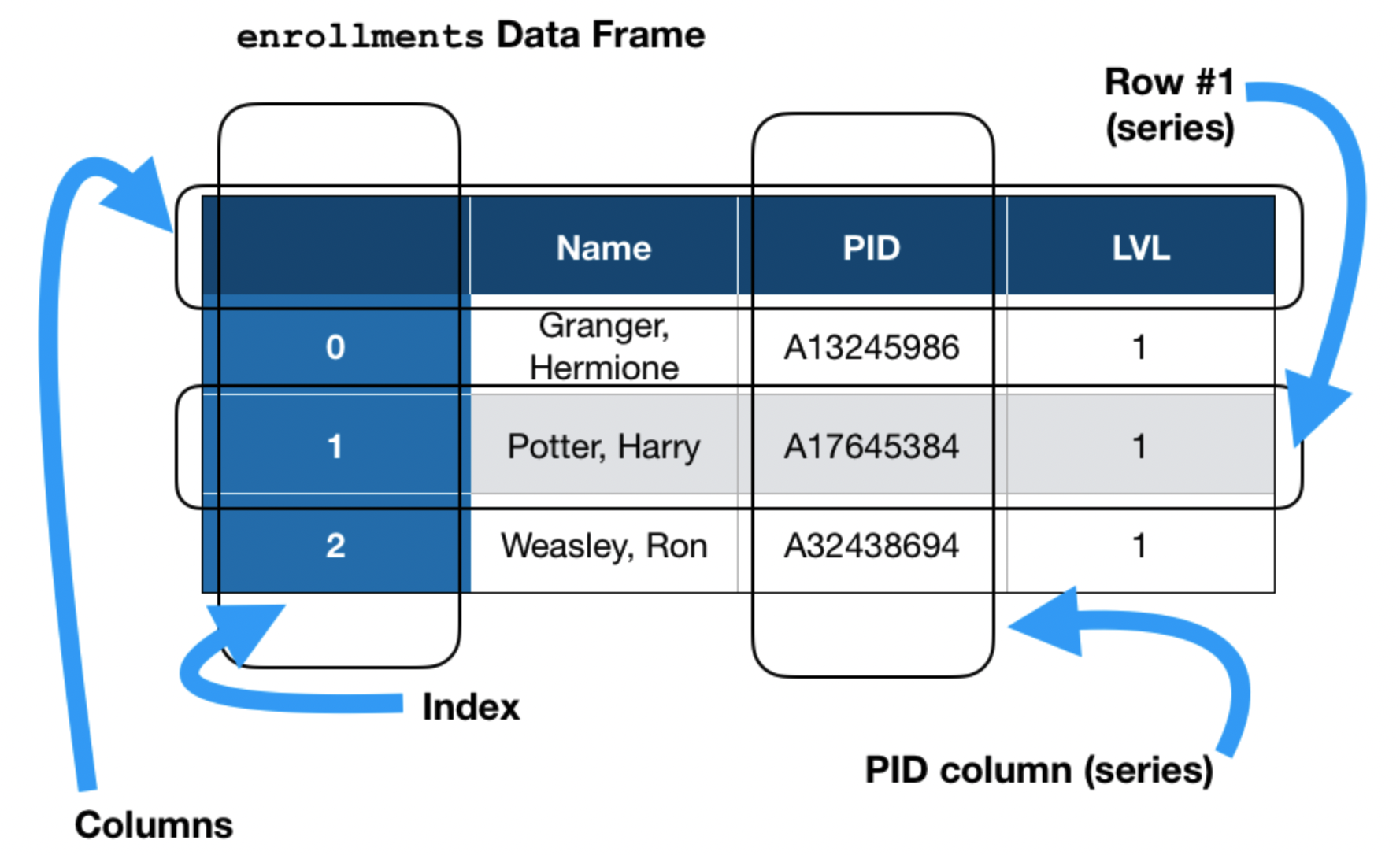
enrollments = pd.DataFrame(column_dict)
enrollments

	Name	PID	LVL
0	Granger, Hermione	A13245986	1
1	Potter, Harry	A17645384	1
2	Weasley, Ron	A32438694	1
3	Longbottom, Neville	A52342436	1

DataFrame index and column labels

• Access column labels with the columns attribute.
• Access index labels with the index attribute.
• The default for both is 0-indexed position (0, 1, 2, ...).

enrollments.columns

Index(['Name', 'PID', 'LVL'], dtype='object')

enrollments.index

RangeIndex(start=0, stop=4, step=1)

Axis

• The rows and columns of a DataFrame are both stored as Series.
• The axis specifies the direction of a slice of a DataFrame.

• Axis 0 refers to the index.
• Axis 1 refers to the columns.

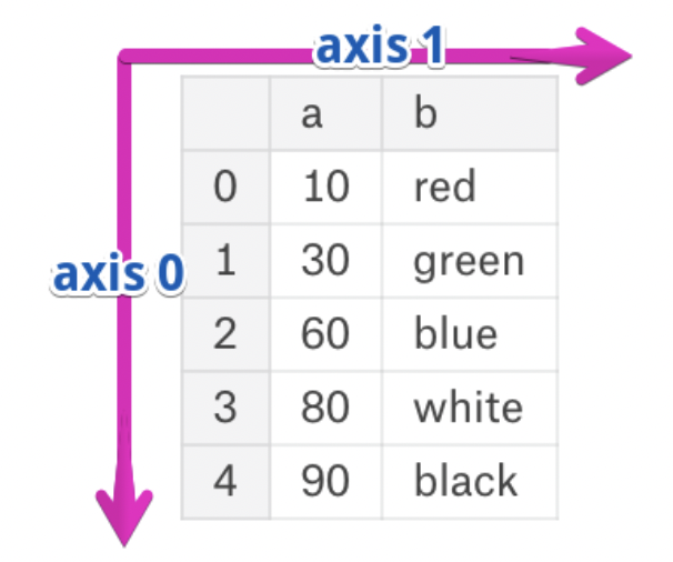
DataFrame methods with axis

A = pd.DataFrame([[1, 2, 3], [4, 5, 6]], columns=['A', 'B', 'C'])
A

	A	B	C
0	1	2	3
1	4	5	6

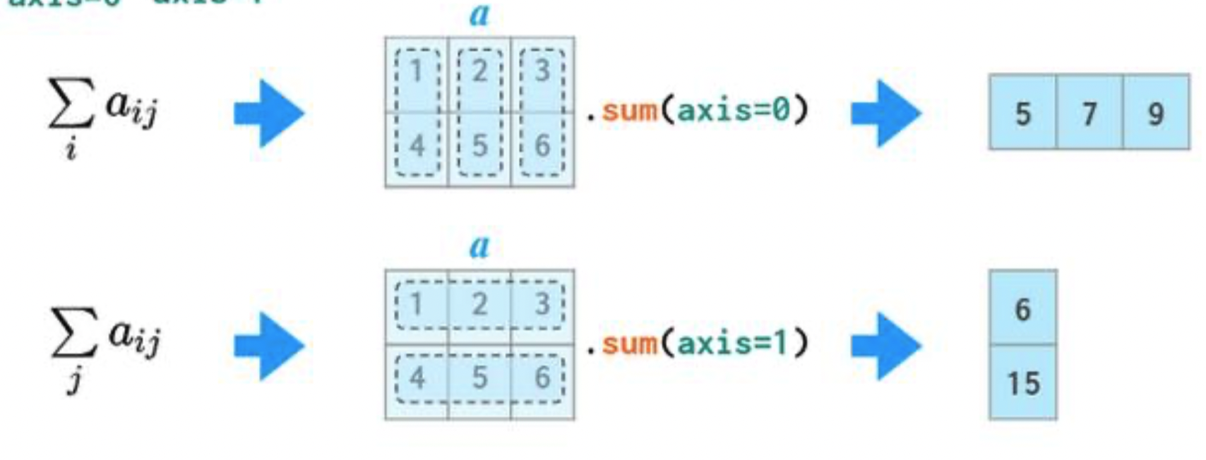
If we specify axis=0, A.sum will "compress" along axis 0, and keep the column labels intact.

A.sum(axis=0)

A    5
B    7
C    9
dtype: int64

If we specify axis=1, A.sum will "compress" along axis 1, and keep the row labels (index) intact.

A.sum(axis=1)

0     6
1    15
dtype: int64

Selecting rows and columns using [] and loc

Throwback to babypandas 👶

• In babypandas, you accessed columns using the .get method.
• .get also works in pandas, but it is not idiomatic – people don't usually use it.

enrollments

	Name	PID	LVL
0	Granger, Hermione	A13245986	1
1	Potter, Harry	A17645384	1
2	Weasley, Ron	A32438694	1
3	Longbottom, Neville	A52342436	1

enrollments.get('Name')

0      Granger, Hermione
1          Potter, Harry
2           Weasley, Ron
3    Longbottom, Neville
Name: Name, dtype: object

# Doesn't error
enrollments.get('billy')

Selecting columns with []

• The standard way to access a column in pandas is by using the [] operator.
  • Think of a DataFrame as a dictionary of arrays!
• Specifying a column name returns the column as a Series.
• Specifying a list of column names returns a DataFrame.

enrollments

	Name	PID	LVL
0	Granger, Hermione	A13245986	1
1	Potter, Harry	A17645384	1
2	Weasley, Ron	A32438694	1
3	Longbottom, Neville	A52342436	1

# Returns a Series
enrollments['Name']

0      Granger, Hermione
1          Potter, Harry
2           Weasley, Ron
3    Longbottom, Neville
Name: Name, dtype: object

# Returns a DataFrame
enrollments[['Name', 'PID']]

	Name	PID
0	Granger, Hermione	A13245986
1	Potter, Harry	A17645384
2	Weasley, Ron	A32438694
3	Longbottom, Neville	A52342436

# 🤔
enrollments[['Name']]

	Name
0	Granger, Hermione
1	Potter, Harry
2	Weasley, Ron
3	Longbottom, Neville

# KeyError
enrollments['billy']

---------------------------------------------------------------------------
KeyError                                  Traceback (most recent call last)
~/opt/anaconda3/lib/python3.9/site-packages/pandas/core/indexes/base.py in get_loc(self, key, method, tolerance)
   3360             try:
-> 3361                 return self._engine.get_loc(casted_key)
   3362             except KeyError as err:

~/opt/anaconda3/lib/python3.9/site-packages/pandas/_libs/index.pyx in pandas._libs.index.IndexEngine.get_loc()

~/opt/anaconda3/lib/python3.9/site-packages/pandas/_libs/index.pyx in pandas._libs.index.IndexEngine.get_loc()

pandas/_libs/hashtable_class_helper.pxi in pandas._libs.hashtable.PyObjectHashTable.get_item()

pandas/_libs/hashtable_class_helper.pxi in pandas._libs.hashtable.PyObjectHashTable.get_item()

KeyError: 'billy'

The above exception was the direct cause of the following exception:

KeyError                                  Traceback (most recent call last)
/var/folders/pd/w73mdrsj2836_7gp0brr2q7r0000gn/T/ipykernel_49367/2071819993.py in <module>
      1 # KeyError
----> 2 enrollments['billy']

~/opt/anaconda3/lib/python3.9/site-packages/pandas/core/frame.py in __getitem__(self, key)
   3456             if self.columns.nlevels > 1:
   3457                 return self._getitem_multilevel(key)
-> 3458             indexer = self.columns.get_loc(key)
   3459             if is_integer(indexer):
   3460                 indexer = [indexer]

~/opt/anaconda3/lib/python3.9/site-packages/pandas/core/indexes/base.py in get_loc(self, key, method, tolerance)
   3361                 return self._engine.get_loc(casted_key)
   3362             except KeyError as err:
-> 3363                 raise KeyError(key) from err
   3364 
   3365         if is_scalar(key) and isna(key) and not self.hasnans:

KeyError: 'billy'

Selecting columns with attribute notation

• It is also possible to access columns using attribute notation, i.e. .<column name>.
• Don't do this.
  • What if the column name clashes with a DataFrame method, like .mean?
  • What if the column name contains spaces or special characters?

enrollments.LVL

0    1
1    1
2    1
3    1
Name: LVL, dtype: int64

enrollments.mean

<bound method NDFrame._add_numeric_operations.<locals>.mean of                   Name        PID  LVL
0    Granger, Hermione  A13245986    1
1        Potter, Harry  A17645384    1
2         Weasley, Ron  A32438694    1
3  Longbottom, Neville  A52342436    1>

Selecting rows with loc

If df is a DataFrame, then:

• df.loc[idx] returns the Series whose index is idx.
• df.loc[idx_list] returns a DataFrame containing the rows whose indexes are in idx_list.

enrollments

	Name	PID	LVL
0	Granger, Hermione	A13245986	1
1	Potter, Harry	A17645384	1
2	Weasley, Ron	A32438694	1
3	Longbottom, Neville	A52342436	1

enrollments.loc[3]

Name    Longbottom, Neville
PID               A52342436
LVL                       1
Name: 3, dtype: object

enrollments.loc[[1, 3]]

	Name	PID	LVL
1	Potter, Harry	A17645384	1
3	Longbottom, Neville	A52342436	1

enrollments.loc[[3]]

	Name	PID	LVL
3	Longbottom, Neville	A52342436	1

Boolean sequence selection

• The loc operator also supports Boolean sequences (lists, arrays, Series) as input.
• The length of the sequence must be the same as the number of rows in the DataFrame.
• The result is a filtered DataFrame, containing only the rows in which the sequence contained True.

enrollments

	Name	PID	LVL
0	Granger, Hermione	A13245986	1
1	Potter, Harry	A17645384	1
2	Weasley, Ron	A32438694	1
3	Longbottom, Neville	A52342436	1

bool_arr = [
    False,  # Hermione
    True,   # Harry
    False,  # Ron
    True    # Neville
]

enrollments.loc[bool_arr]

	Name	PID	LVL
1	Potter, Harry	A17645384	1
3	Longbottom, Neville	A52342436	1

Querying

• Comparisons with arrays (Series) result in Boolean arrays (Series).
• We can use comparisons along with the loc operator to query a DataFrame.
• Querying is the act of selecting rows in a DataFrame that satisfy certain condition(s).

enrollments

	Name	PID	LVL
0	Granger, Hermione	A13245986	1
1	Potter, Harry	A17645384	1
2	Weasley, Ron	A32438694	1
3	Longbottom, Neville	A52342436	1

enrollments['Name'].str.contains('on')

0     True
1    False
2     True
3     True
Name: Name, dtype: bool

# Rows where Name includes 'on'
enrollments.loc[enrollments['Name'].str.contains('on')]

	Name	PID	LVL
0	Granger, Hermione	A13245986	1
2	Weasley, Ron	A32438694	1
3	Longbottom, Neville	A52342436	1

# Rows where the first letter of Name is between A and L
enrollments.loc[enrollments['Name'] < 'M']

	Name	PID	LVL
0	Granger, Hermione	A13245986	1
3	Longbottom, Neville	A52342436	1

When using a Boolean sequence, e.g. enrollments['Name'] < 'M', loc is not strictly necessary:

enrollments[enrollments['Name'] < 'M']

	Name	PID	LVL
0	Granger, Hermione	A13245986	1
3	Longbottom, Neville	A52342436	1

Selecting columns and rows simultaneously

So far, we used [] to select columns and loc to select rows.

enrollments.loc[enrollments['Name'] < 'M']['PID']

0    A13245986
3    A52342436
Name: PID, dtype: object

Selecting columns and rows simultaneously

loc can also be used to select both rows and columns. The general pattern is:

df.loc[<row selector>, <column selector>]

Examples:

• df.loc[idx_list, col_list] returns a DataFrame containing the rows in idx_list and columns in col_list.
• df.loc[bool_arr, col_list] returns a DataFrame contaning the rows for which bool_arr is True and columns in col_list.
• If : is used as the first input, all rows are kept. If : is used as the second input, all columns are kept.

enrollments

	Name	PID	LVL
0	Granger, Hermione	A13245986	1
1	Potter, Harry	A17645384	1
2	Weasley, Ron	A32438694	1
3	Longbottom, Neville	A52342436	1

enrollments.loc[enrollments['Name'] < 'M', 'PID']

0    A13245986
3    A52342436
Name: PID, dtype: object

enrollments.loc[enrollments['Name'] < 'M', ['PID']]

	PID
0	A13245986
3	A52342436

Even more ways of selecting rows and columns

In df.loc[<row selection>, <column selection>]:

• Both the first and second inputs can be Boolean sequences.
• Both the first and second inputs can be slices, which use : syntax (e.g. 0:2, 'Name': 'PID').
• If both the first and second inputs are primitives (strings or numbers), the result is a single value, not a DataFrame or Series.
• The first input can be a function that takes a row as input and returns a Boolean.

There are many, many more – see the pandas documentation for more.

enrollments

	Name	PID	LVL
0	Granger, Hermione	A13245986	1
1	Potter, Harry	A17645384	1
2	Weasley, Ron	A32438694	1
3	Longbottom, Neville	A52342436	1

enrollments.loc[2, 'LVL']

1

enrollments.loc[0:2, 'Name': 'PID']

	Name	PID
0	Granger, Hermione	A13245986
1	Potter, Harry	A17645384
2	Weasley, Ron	A32438694

Don't forget iloc!

• iloc stands for "integer location".
• iloc is like loc, but it selects rows and columns based off of integer positions only.

enrollments

	Name	PID	LVL
0	Granger, Hermione	A13245986	1
1	Potter, Harry	A17645384	1
2	Weasley, Ron	A32438694	1
3	Longbottom, Neville	A52342436	1

enrollments.iloc[2:4, 0:2]

	Name	PID
2	Weasley, Ron	A32438694
3	Longbottom, Neville	A52342436

other = enrollments.set_index('Name')
other

	PID	LVL
Name
Granger, Hermione	A13245986	1
Potter, Harry	A17645384	1
Weasley, Ron	A32438694	1
Longbottom, Neville	A52342436	1

other.iloc[2]

PID    A32438694
LVL            1
Name: Weasley, Ron, dtype: object

other.loc[2]

---------------------------------------------------------------------------
KeyError                                  Traceback (most recent call last)
~/opt/anaconda3/lib/python3.9/site-packages/pandas/core/indexes/base.py in get_loc(self, key, method, tolerance)
   3360             try:
-> 3361                 return self._engine.get_loc(casted_key)
   3362             except KeyError as err:

~/opt/anaconda3/lib/python3.9/site-packages/pandas/_libs/index.pyx in pandas._libs.index.IndexEngine.get_loc()

~/opt/anaconda3/lib/python3.9/site-packages/pandas/_libs/index.pyx in pandas._libs.index.IndexEngine.get_loc()

pandas/_libs/hashtable_class_helper.pxi in pandas._libs.hashtable.PyObjectHashTable.get_item()

pandas/_libs/hashtable_class_helper.pxi in pandas._libs.hashtable.PyObjectHashTable.get_item()

KeyError: 2

The above exception was the direct cause of the following exception:

KeyError                                  Traceback (most recent call last)
/var/folders/pd/w73mdrsj2836_7gp0brr2q7r0000gn/T/ipykernel_49367/776803957.py in <module>
----> 1 other.loc[2]

~/opt/anaconda3/lib/python3.9/site-packages/pandas/core/indexing.py in __getitem__(self, key)
    929 
    930             maybe_callable = com.apply_if_callable(key, self.obj)
--> 931             return self._getitem_axis(maybe_callable, axis=axis)
    932 
    933     def _is_scalar_access(self, key: tuple):

~/opt/anaconda3/lib/python3.9/site-packages/pandas/core/indexing.py in _getitem_axis(self, key, axis)
   1162         # fall thru to straight lookup
   1163         self._validate_key(key, axis)
-> 1164         return self._get_label(key, axis=axis)
   1165 
   1166     def _get_slice_axis(self, slice_obj: slice, axis: int):

~/opt/anaconda3/lib/python3.9/site-packages/pandas/core/indexing.py in _get_label(self, label, axis)
   1111     def _get_label(self, label, axis: int):
   1112         # GH#5667 this will fail if the label is not present in the axis.
-> 1113         return self.obj.xs(label, axis=axis)
   1114 
   1115     def _handle_lowerdim_multi_index_axis0(self, tup: tuple):

~/opt/anaconda3/lib/python3.9/site-packages/pandas/core/generic.py in xs(self, key, axis, level, drop_level)
   3774                 raise TypeError(f"Expected label or tuple of labels, got {key}") from e
   3775         else:
-> 3776             loc = index.get_loc(key)
   3777 
   3778             if isinstance(loc, np.ndarray):

~/opt/anaconda3/lib/python3.9/site-packages/pandas/core/indexes/base.py in get_loc(self, key, method, tolerance)
   3361                 return self._engine.get_loc(casted_key)
   3362             except KeyError as err:
-> 3363                 raise KeyError(key) from err
   3364 
   3365         if is_scalar(key) and isna(key) and not self.hasnans:

KeyError: 2

Discussion Question

Let's return to the names DataFrame.

names

	firstname	gender	count	year
0	Emily	F	25957	2000
1	Hannah	F	23084	2000
2	Madison	F	19968	2000
3	Ashley	F	17997	2000
4	Sarah	F	17706	2000
...	...	...	...	...
32025	Zyheem	M	5	2019
32026	Zykel	M	5	2019
32027	Zyking	M	5	2019
32028	Zyn	M	5	2019
32029	Zyran	M	5	2019

1399746 rows × 4 columns

Question: How many babies were born with the name 'Billy' and gender 'M'?

...

More Practice

Consider the DataFrame below.

jack = pd.DataFrame({1: ['fee', 'fi'], '1': ['fo', 'fum']})
jack

For each of the following pieces of code, predict what the output will be. Then, uncomment the line of code and see for yourself.

# jack[1]

# jack[[1]]

# jack['1']

# jack[[1,1]]

# jack.loc[1]

# jack.loc[jack[1] == 'fo']

# jack[1, ['1', 1]]

# jack.loc[1,1]

Summary, next time

Summary

• pandas is the library for tabular data manipulation in Python.
• There are three key data structures in pandas: DataFrame, Series, and Index.
• Refer to the lecture notebook and the pandas documentation for tips.
• Next time: useful methods for working with DataFrames and Series.