import pandas as pd
import numpy as np
import os

Lecture 9 – Combining Data

DSC 80, Spring 2022

Announcements

• Discussion 3 is due (for extra credit!) tomorrow at 11:59PM.
• Lab 3 is due on Monday, April 18th 11:59PM.
  • Check here for clarifications.
• Lab 1 (+more) grades are released – see this post for details, and this post for assignment solutions.
• Watch this video 🎥 for tips on how to work with the command-line.
• Project 2 will be released this weekend.

Agenda

• Concatenating vertically.
• Concatenating horizontally.
• Joining and merging.
• Working with time series data.

Good resource: pandas User Guide.

Recap: Concatenating vertically

Example: Grades

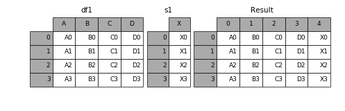
By default, pd.concat stacks DataFrames row-wise, i.e. on top of one another.

section_A = pd.DataFrame({
    'Name': ['Annie', 'Billy', 'Sally', 'Tommy'],
    'Midterm': [98, 82, 23, 45],
    'Final': [88, 100, 99, 67]
})

section_A

	Name	Midterm	Final
0	Annie	98	88
1	Billy	82	100
2	Sally	23	99
3	Tommy	45	67

section_B = pd.DataFrame({
    'Name': ['Junior', 'Rex', 'Flash'],
    'Midterm': [70, 99, 81],
    'Final': [42, 25, 90]
})

section_B

	Name	Midterm	Final
0	Junior	70	42
1	Rex	99	25
2	Flash	81	90

Let's use pd.concat on a list of the above two DataFrames.

pd.concat([section_A, section_B])

	Name	Midterm	Final
0	Annie	98	88
1	Billy	82	100
2	Sally	23	99
3	Tommy	45	67
0	Junior	70	42
1	Rex	99	25
2	Flash	81	90

⚠️ Warning: No loops!

• pd.concat returns a copy; it does not modify any of the input DataFrames.
• Do not use pd.concat in a loop, as it has terrible time and space efficiency.

total = pd.DataFrame()
for df in dataframes:
    total = total.concat(df)

• Instead, use pd.concat(dataframes), where dataframes is a list of DataFrames.

Concatenating horizontally

Example: Grades (again)

Suppose we have two DataFrames, exams and assignments, which both contain different attributes for the same individuals.

exams = section_A.copy()
exams

	Name	Midterm	Final
0	Annie	98	88
1	Billy	82	100
2	Sally	23	99
3	Tommy	45	67

assignments = exams[['Name']].assign(Homeworks=[99, 45, 23, 81],
                                     Labs=[100, 100, 99, 100])

assignments

	Name	Homeworks	Labs
0	Annie	99	100
1	Billy	45	100
2	Sally	23	99
3	Tommy	81	100

If we try to combine these DataFrames with pd.concat, we don't quite get what we're looking for.

pd.concat([exams, assignments])

	Name	Midterm	Final	Homeworks	Labs
0	Annie	98.0	88.0	NaN	NaN
1	Billy	82.0	100.0	NaN	NaN
2	Sally	23.0	99.0	NaN	NaN
3	Tommy	45.0	67.0	NaN	NaN
0	Annie	NaN	NaN	99.0	100.0
1	Billy	NaN	NaN	45.0	100.0
2	Sally	NaN	NaN	23.0	99.0
3	Tommy	NaN	NaN	81.0	100.0

But that's where the axis argument becomes handy.

Remember, most pandas operations default to axis=0, but here we want to concatenate the columns of exams to the columns of assignments, so we should use axis=1.

pd.concat([exams, assignments], axis=1)

	Name	Midterm	Final	Name	Homeworks	Labs
0	Annie	98	88	Annie	99	100
1	Billy	82	100	Billy	45	100
2	Sally	23	99	Sally	23	99
3	Tommy	45	67	Tommy	81	100

Note that the 'Name' column appears twice!

Concatenating horizontally

• To concatenate two DataFrames horizontally, use pd.concat with axis=1.
• Concatenation is done by matching indexes, regardless of their order. It does not look at any column values!

Note that the call to pd.concat below works as expected, even though the orders of the names in exams_by_name and assignments_by_name are different.

# .loc[::-1] reverses the rows of the DataFrame
exams_by_name = exams.set_index('Name').loc[::-1]
exams_by_name

	Midterm	Final
Name
Tommy	45	67
Sally	23	99
Billy	82	100
Annie	98	88

assignments_by_name = assignments.set_index('Name')
assignments_by_name

	Homeworks	Labs
Name
Annie	99	100
Billy	45	100
Sally	23	99
Tommy	81	100

pd.concat([exams_by_name, assignments_by_name], axis=1)

	Midterm	Final	Homeworks	Labs
Name
Tommy	45	67	81	100
Sally	23	99	23	99
Billy	82	100	45	100
Annie	98	88	99	100

Remember that pd.concat only looks at the index when combining rows, not at any other columns.

exams_reversed = exams.loc[::-1].reset_index(drop=True)
exams_reversed

	Name	Midterm	Final
0	Tommy	45	67
1	Sally	23	99
2	Billy	82	100
3	Annie	98	88

assignments

	Name	Homeworks	Labs
0	Annie	99	100
1	Billy	45	100
2	Sally	23	99
3	Tommy	81	100

pd.concat([exams_reversed, assignments], axis=1)

	Name	Midterm	Final	Name	Homeworks	Labs
0	Tommy	45	67	Annie	99	100
1	Sally	23	99	Billy	45	100
2	Billy	82	100	Sally	23	99
3	Annie	98	88	Tommy	81	100

Missing rows?

If we concatenate two DataFrames that don't share row indexes, NaNs are added in the rows that aren't shared.

exams_extra = exams.copy()
exams_extra.loc[4] = ['Junior', 100, 100]
exams_extra

	Name	Midterm	Final
0	Annie	98	88
1	Billy	82	100
2	Sally	23	99
3	Tommy	45	67
4	Junior	100	100

assignments

	Name	Homeworks	Labs
0	Annie	99	100
1	Billy	45	100
2	Sally	23	99
3	Tommy	81	100

pd.concat([exams_extra, assignments], axis=1)

	Name	Midterm	Final	Name	Homeworks	Labs
0	Annie	98	88	Annie	99.0	100.0
1	Billy	82	100	Billy	45.0	100.0
2	Sally	23	99	Sally	23.0	99.0
3	Tommy	45	67	Tommy	81.0	100.0
4	Junior	100	100	NaN	NaN	NaN

Summary: pd.concat

• pd.concat "stitches" two or more DataFrames together.
• If you use axis=0, the DataFrames are concatenated vertically based on column names (rows on top of rows).
• If you use axis=1, the DataFrames are concatenated horizontally based on row indexes (columns next to columns).

Joining and merging

Concatenating horizontally

• pd.concat with axis=1 combines DataFrames horizontally.
• To combine DataFrames horizontally in more advanced ways, we perform a join (also known as a merge).

Joins

• A join creates a new DataFrame by combining the rows of two DataFrames.
• A join is appropriate when we have two sources of information
  • about the same individuals, that is
  • linked by a common column.
• The common column is called the join key.

Example

Here, the join key is 'Player Id'.

The merge method

• The merge DataFrame method joins two tables by columns or indexes.
  • "Merge" is just pandas' word for "join".
  • It also exists as a pandas function.
• If join keys are not specified, all shared columns between the two DataFrames are used by default.

Let's work with a small example.

temps = pd.DataFrame({
    'City': ['San Diego', 'Toronto', 'Rome'],
    'Temperature': [76, 28, 56]
})

temps

	City	Temperature
0	San Diego	76
1	Toronto	28
2	Rome	56

countries = pd.DataFrame({
    'City': ['Toronto', 'Shanghai', 'San Diego'],
    'Country': ['Canada', 'China', 'USA']
})

countries

	City	Country
0	Toronto	Canada
1	Shanghai	China
2	San Diego	USA

temps.merge(countries)

	City	Temperature	Country
0	San Diego	76	USA
1	Toronto	28	Canada

We didn't specify which columns to merge on, so it defaulted to 'City'.

Join types: inner joins

• Note that 'Rome' and 'Shanghai' do not appear in the merged DataFrame.
• This is because there is:
  • no city named 'Rome' in the second DataFrame, and
  • no city named 'Shanghai' in the first DataFrame.
• The default type of join that merge performs is an inner join, which keeps the intersection of the join keys.

Different join types handle mismatches differently

There are four types of joins.

• Inner: keep only matching keys (intersection).
• Outer: keeps all keys in both DataFrames (union).
• Left: keep all keys in the left DataFrame, whether or not they are in the right DataFrame.
• Right: keep all keys in the right DataFrame, whether or not they are in the left DataFrame.

Examples of join types

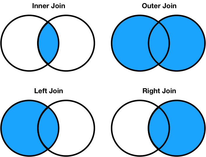
• To specify which type of join we want to perform, we use the how argument (the default is how='inner').
• The left DataFrame is the DataFrame that preceeds .merge, and the right DataFrame is the argument to merge.
• Alternatively, you can use the pd.merge function, in which the first argument is the left DataFrame and the second argument is the right DataFrame.

temps

	City	Temperature
0	San Diego	76
1	Toronto	28
2	Rome	56

countries

	City	Country
0	Toronto	Canada
1	Shanghai	China
2	San Diego	USA

Let's try an outer join.

temps.merge(countries, how='outer')

	City	Temperature	Country
0	San Diego	76.0	USA
1	Toronto	28.0	Canada
2	Rome	56.0	NaN
3	Shanghai	NaN	China

# merge is also a pandas function
pd.merge(temps, countries, how='outer')

	City	Temperature	Country
0	San Diego	76.0	USA
1	Toronto	28.0	Canada
2	Rome	56.0	NaN
3	Shanghai	NaN	China

Note the NaNs in the rows for 'Rome' and 'Shanghai'.

Also note that an outer join is what pd.concat does by default, when there are no duplicated keys in either DataFrame.

pd.concat([temps.set_index('City'), countries.set_index('City')], axis=1)

	Temperature	Country
City
San Diego	76.0	USA
Toronto	28.0	Canada
Rome	56.0	NaN
Shanghai	NaN	China

Let's try left and right joins.

temps

	City	Temperature
0	San Diego	76
1	Toronto	28
2	Rome	56

countries

	City	Country
0	Toronto	Canada
1	Shanghai	China
2	San Diego	USA

First, a left join.

temps.merge(countries, how='left')

	City	Temperature	Country
0	San Diego	76	USA
1	Toronto	28	Canada
2	Rome	56	NaN

How about a right join?

temps.merge(countries, how='right')

	City	Temperature	Country
0	Toronto	28.0	Canada
1	Shanghai	NaN	China
2	San Diego	76.0	USA

Note that a.merge(b, how='left') is the same as b.merge(a, how='right'). The only difference is the order of the columns in the result.

countries.merge(temps, how='left')

	City	Country	Temperature
0	Toronto	Canada	28.0
1	Shanghai	China	NaN
2	San Diego	USA	76.0

Specifying join keys

• pandas defaults to using the shared column(s) as join keys.
• If there are multiple shared column names and you only want to join on one of them, or if there are no shared column names, then you will need to specify which columns to join on.
• Two solutions:
  1. Use the on argument if the desired column(s) have the same names in both DataFrames.
  2. Use the left_on or left_index argument AND the right_on or right_index argument.

exams

	Name	Midterm	Final
0	Annie	98	88
1	Billy	82	100
2	Sally	23	99
3	Tommy	45	67

overall = pd.DataFrame({
    'PID': ['A15253545', 'A10348245', 'A13349069', 'A18485824', 'A10094857'],
    'Student': ['Billy', 'Sally', 'Annie', 'Larry', 'Johnny'],
    'Final': [88, 64, 91, 45, 89]
})

overall

	PID	Student	Final
0	A15253545	Billy	88
1	A10348245	Sally	64
2	A13349069	Annie	91
3	A18485824	Larry	45
4	A10094857	Johnny	89

This is not what we're looking for.

exams.merge(overall)

	Name	Midterm	Final	PID	Student
0	Annie	98	88	A15253545	Billy

Instead, we need to tell pandas to look in the 'Name' column of exams and 'Student' column of overall.

exams.merge(overall, left_on='Name', right_on='Student')

	Name	Midterm	Final_x	PID	Student	Final_y
0	Annie	98	88	A13349069	Annie	91
1	Billy	82	100	A15253545	Billy	88
2	Sally	23	99	A10348245	Sally	64

If there are shared column names in the two DataFrames you are merging that you are not using as join keys, by default '_x' and '_y' are appended to their names.

exams.merge(overall, left_on='Name', right_on='Student', suffixes=('_Exam', '_Overall'))

	Name	Midterm	Final_Exam	PID	Student	Final_Overall
0	Annie	98	88	A13349069	Annie	91
1	Billy	82	100	A15253545	Billy	88
2	Sally	23	99	A10348245	Sally	64

If the desired join key is in the index, assign left_index or right_index to True.

exams

	Name	Midterm	Final
0	Annie	98	88
1	Billy	82	100
2	Sally	23	99
3	Tommy	45	67

overall_by_student = overall.set_index('Student')
overall_by_student

	PID	Final
Student
Billy	A15253545	88
Sally	A10348245	64
Annie	A13349069	91
Larry	A18485824	45
Johnny	A10094857	89

exams.merge(overall_by_student, left_on='Name', right_index=True, suffixes=('_Exam', '_Overall'))

	Name	Midterm	Final_Exam	PID	Final_Overall
0	Annie	98	88	A13349069	91
1	Billy	82	100	A15253545	88
2	Sally	23	99	A10348245	64

Many-to-one & many-to-many joins

One-to-one joins

• So far in this lecture, the joins we have worked with are called one-to-one joins.
• Neither the left DataFrame nor the right DataFrame contained any duplicates in the join key.
• What if there are duplicated join keys, in one or both of the DataFrames we are merging?

Many-to-one joins

• Many-to-one joins are joins where one of the DataFrames contains duplicate values in the join key.
• The resulting DataFrame will preserve those duplicate entries as appropriate.

profs = pd.DataFrame(
[['Brad', 'UCB', 8],
 ['Janine', 'UCSD', 7],
 ['Marina', 'UIC', 6],
 ['Justin', 'OSU', 4],
 ['Aaron', 'UCB', 4],
 ['Soohyun', 'UCSD', 1],
 ['Suraj', 'UCB', 1]],
    columns=['Name', 'School', 'Years']
)

profs

	Name	School	Years
0	Brad	UCB	8
1	Janine	UCSD	7
2	Marina	UIC	6
3	Justin	OSU	4
4	Aaron	UCB	4
5	Soohyun	UCSD	1
6	Suraj	UCB	1

schools = pd.DataFrame({
    'Abr': ['UCSD', 'UCLA', 'UCB', 'UIC'],
    'Full': ['University of California, San Diego', 'University of California, Los Angeles', 'University of California, Berkeley', 'University of Illinois Chicago']
})

schools

	Abr	Full
0	UCSD	University of California, San Diego
1	UCLA	University of California, Los Angeles
2	UCB	University of California, Berkeley
3	UIC	University of Illinois Chicago

Note that when merging profs and schools, the information from schools is duplicated ('University of California, San Diego' appears twice and 'University of California, Berkeley' appears three times).

profs.merge(schools, left_on='School', right_on='Abr', how='left')

	Name	School	Years	Abr	Full
0	Brad	UCB	8	UCB	University of California, Berkeley
1	Janine	UCSD	7	UCSD	University of California, San Diego
2	Marina	UIC	6	UIC	University of Illinois Chicago
3	Justin	OSU	4	NaN	NaN
4	Aaron	UCB	4	UCB	University of California, Berkeley
5	Soohyun	UCSD	1	UCSD	University of California, San Diego
6	Suraj	UCB	1	UCB	University of California, Berkeley

Many-to-many joins

Many-to-many joins are joins where both DataFrames have duplicate values in the join key.

profs

	Name	School	Years
0	Brad	UCB	8
1	Janine	UCSD	7
2	Marina	UIC	6
3	Justin	OSU	4
4	Aaron	UCB	4
5	Soohyun	UCSD	1
6	Suraj	UCB	1

programs = pd.DataFrame({
    'uni': ['UCSD', 'UCSD', 'UCSD', 'UCB', 'OSU', 'OSU'],
    'dept': ['Math', 'HDSI', 'COGS', 'CS', 'Math', 'CS'],
    'grad_students': [205, 54, 281, 439, 304, 193]
})

programs

	uni	dept	grad_students
0	UCSD	Math	205
1	UCSD	HDSI	54
2	UCSD	COGS	281
3	UCB	CS	439
4	OSU	Math	304
5	OSU	CS	193

Before running the following cell, try predicting the number of rows in the output.

profs.merge(programs, left_on='School', right_on='uni')

	Name	School	Years	uni	dept	grad_students
0	Brad	UCB	8	UCB	CS	439
1	Aaron	UCB	4	UCB	CS	439
2	Suraj	UCB	1	UCB	CS	439
3	Janine	UCSD	7	UCSD	Math	205
4	Janine	UCSD	7	UCSD	HDSI	54
5	Janine	UCSD	7	UCSD	COGS	281
6	Soohyun	UCSD	1	UCSD	Math	205
7	Soohyun	UCSD	1	UCSD	HDSI	54
8	Soohyun	UCSD	1	UCSD	COGS	281
9	Justin	OSU	4	OSU	Math	304
10	Justin	OSU	4	OSU	CS	193

• merge stitched together every UCSD row in profs with every UCSD row in programs.
• Since there were 2 UCSD rows in profs and 3 in programs, there are $2 \cdot 3 = 6$ UCSD rows in the output. The same applies for all other schools.

Example: SDPD vehicle stops

Aside: accessing file names programmatically

• At times, you'll need to load in all of the files in a given folder.
• os.listdir(dirname) returns a list of the names of the files in the folder dirname.

os.listdir('data')

['orders.csv',
 '.DS_Store',
 'stops_2017.csv',
 'military.csv',
 'stops_2016.csv',
 'race_codes.csv']

• Sometimes, you'll want to extract file names that follow a specific pattern. The pathlib library allows you to do this.

import pathlib
file_list = list(pathlib.Path().glob('data/stops*.csv')) # glob allows for pattern matching
file_list

[PosixPath('data/stops_2017.csv'), PosixPath('data/stops_2016.csv')]

• You can accomplish something similar in the command-line.
• Place a ! in front of a command in a Jupyter Notebook cell to run it on the command-line.

!ls data/stops*.csv

data/stops_2016.csv data/stops_2017.csv

Loading in the data

file_list

[PosixPath('data/stops_2017.csv'), PosixPath('data/stops_2016.csv')]

list_of_dfs = [pd.read_csv(file) for file in file_list]

for df in list_of_dfs:
    display(df.head())

	stop_id	stop_cause	service_area	subject_race	subject_sex	subject_age	timestamp	stop_date	stop_time	sd_resident	arrested	searched	obtained_consent	contraband_found	property_seized
0	1444799	Moving Violation	120	I	M	37	2017-01-01 00:03:00	2017-01-01	00:03:00	N	N	N	NaN	NaN	NaN
1	1444821	Equipment Violation	520	W	M	22	2017-01-01 00:25:00	2017-01-01	00:25:00	N	N	N	NaN	NaN	NaN
2	1447102	Moving Violation	520	W	M	29	2017-01-01 01:45:00	2017-01-01	01:45:00	N	N	N	NaN	NaN	NaN
3	1444801	Equipment Violation	720	H	F	61	2017-01-01 03:10:00	2017-01-01	03:10:00	N	N	N	NaN	NaN	NaN
4	1444802	Equipment Violation	120	H	M	24	2017-01-01 03:30:00	2017-01-01	03:30:00	Y	N	N	NaN	NaN	NaN

	stop_id	stop_cause	service_area	subject_race	subject_sex	subject_age	timestamp	stop_date	stop_time	sd_resident	arrested	searched	obtained_consent	contraband_found	property_seized
0	1308198	Equipment Violation	530	W	M	28	2016-01-01 00:06:00	2016-01-01	0:06	Y	N	N	N	N	N
1	1308172	Moving Violation	520	B	M	25	2016-01-01 00:10:00	2016-01-01	0:10	N	N	N	NaN	NaN	NaN
2	1308171	Moving Violation	110	H	F	31	2016-01-01 00:14:00	2016-01-01	0:14	NaN	NaN	NaN	NaN	NaN	NaN
3	1308170	Moving Violation	Unknown	W	F	29	2016-01-01 00:16:00	2016-01-01	0:16	N	N	N	NaN	NaN	NaN
4	1308197	Moving Violation	230	W	M	52	2016-01-01 00:30:00	2016-01-01	0:30	N	N	N	NaN	NaN	NaN

We need to concatenate these two DataFrames vertically.

stops = pd.concat(list_of_dfs, ignore_index=True)

stops.head()

	stop_id	stop_cause	service_area	subject_race	subject_sex	subject_age	timestamp	stop_date	stop_time	sd_resident	arrested	searched	obtained_consent	contraband_found	property_seized
0	1444799	Moving Violation	120	I	M	37	2017-01-01 00:03:00	2017-01-01	00:03:00	N	N	N	NaN	NaN	NaN
1	1444821	Equipment Violation	520	W	M	22	2017-01-01 00:25:00	2017-01-01	00:25:00	N	N	N	NaN	NaN	NaN
2	1447102	Moving Violation	520	W	M	29	2017-01-01 01:45:00	2017-01-01	01:45:00	N	N	N	NaN	NaN	NaN
3	1444801	Equipment Violation	720	H	F	61	2017-01-01 03:10:00	2017-01-01	03:10:00	N	N	N	NaN	NaN	NaN
4	1444802	Equipment Violation	120	H	M	24	2017-01-01 03:30:00	2017-01-01	03:30:00	Y	N	N	NaN	NaN	NaN

len(stops)

206413

Investigating races

Right now, 'subject_race' is stored as a single character. What does 'I' mean? 'H'?

stops.head()

	stop_id	stop_cause	service_area	subject_race	subject_sex	subject_age	timestamp	stop_date	stop_time	sd_resident	arrested	searched	obtained_consent	contraband_found	property_seized
0	1444799	Moving Violation	120	I	M	37	2017-01-01 00:03:00	2017-01-01	00:03:00	N	N	N	NaN	NaN	NaN
1	1444821	Equipment Violation	520	W	M	22	2017-01-01 00:25:00	2017-01-01	00:25:00	N	N	N	NaN	NaN	NaN
2	1447102	Moving Violation	520	W	M	29	2017-01-01 01:45:00	2017-01-01	01:45:00	N	N	N	NaN	NaN	NaN
3	1444801	Equipment Violation	720	H	F	61	2017-01-01 03:10:00	2017-01-01	03:10:00	N	N	N	NaN	NaN	NaN
4	1444802	Equipment Violation	120	H	M	24	2017-01-01 03:30:00	2017-01-01	03:30:00	Y	N	N	NaN	NaN	NaN

stops['subject_race'].value_counts(normalize=True)

W    0.411358
H    0.309249
B    0.112620
O    0.086896
A    0.046397
F    0.011923
V    0.005768
C    0.004899
I    0.004123
X    0.001446
K    0.001222
P    0.000990
J    0.000912
Z    0.000558
D    0.000543
L    0.000461
S    0.000349
G    0.000189
U    0.000097
Name: subject_race, dtype: float64

Fortunately, we have access to another dataset that describes each of the race codes.

races = pd.read_csv('data/race_codes.csv')
races

	Race Code	Description
0	A	OTHER ASIAN
1	B	BLACK
2	C	CHINESE
3	D	CAMBODIAN
4	F	FILIPINO
5	G	GUAMANIAN
6	H	HISPANIC
7	I	INDIAN
8	J	JAPANESE
9	K	KOREAN
10	L	LAOTIAN
11	O	OTHER
12	P	PACIFIC ISLANDER
13	S	SAMOAN
14	U	HAWAIIAN
15	V	VIETNAMESE
16	W	WHITE
17	Z	ASIAN INDIAN

Let's join the distribution of races with the DataFrame of race codes.

Question: Is this a one-to-one join?

race_percentages = stops['subject_race'].value_counts(normalize=True).rename('Proportion').to_frame()
race_percentages.merge(races, left_index=True, right_on='Race Code')

	Proportion	Race Code	Description
16	0.411358	W	WHITE
6	0.309249	H	HISPANIC
1	0.112620	B	BLACK
11	0.086896	O	OTHER
0	0.046397	A	OTHER ASIAN
4	0.011923	F	FILIPINO
15	0.005768	V	VIETNAMESE
2	0.004899	C	CHINESE
7	0.004123	I	INDIAN
9	0.001222	K	KOREAN
12	0.000990	P	PACIFIC ISLANDER
8	0.000912	J	JAPANESE
17	0.000558	Z	ASIAN INDIAN
3	0.000543	D	CAMBODIAN
10	0.000461	L	LAOTIAN
13	0.000349	S	SAMOAN
5	0.000189	G	GUAMANIAN
14	0.000097	U	HAWAIIAN

The level of granularity of the races in our data right now seems inconsistent. For instance, 'WHITE' and 'BLACK' are much more broad than 'FILIPINO', 'JAPANESE', and 'GUAMANIAN'.

Adjusting granularity

Let's try and adjust our race data so that we have a consistent level of granularity. Here's what we want to create:

	Race Code	Description	Race_Category
0	A	OTHER ASIAN	Asian
1	B	BLACK	Black
2	C	CHINESE	Asian
3	D	CAMBODIAN	Asian
4	F	FILIPINO	Asian

We can do this by manually defining a mapping between race codes and desired categories.

race_dict = {'A':'Asian',
             'B':'Black',
             'C':'Asian',
             'D':'Asian',
             'F':'Asian',
             'G':'Asian',
             'H':'Hispanic',
             'I':'Native American',
             'J':'Asian',
             'K':'Asian',
             'L':'Asian',
             'O':'Other',
             'P':'Asian',
             'S':'Asian',
             'U':'Hawaiian',
             'V':'Asian',
             'W':'White',
             'Z':'Asian'
            }

There are two ways to replace all of the 'Race Code's in races with the above categories:

• Use the Series replace method.
• Convert the above mapping to a DataFrame and join it with races.

Joining requires sorting, where as replacing does not. Let's go with the first option.

races['Race_Category'] = races['Race Code'].replace(race_dict)
races

	Race Code	Description	Race_Category
0	A	OTHER ASIAN	Asian
1	B	BLACK	Black
2	C	CHINESE	Asian
3	D	CAMBODIAN	Asian
4	F	FILIPINO	Asian
5	G	GUAMANIAN	Asian
6	H	HISPANIC	Hispanic
7	I	INDIAN	Native American
8	J	JAPANESE	Asian
9	K	KOREAN	Asian
10	L	LAOTIAN	Asian
11	O	OTHER	Other
12	P	PACIFIC ISLANDER	Asian
13	S	SAMOAN	Asian
14	U	HAWAIIAN	Hawaiian
15	V	VIETNAMESE	Asian
16	W	WHITE	White
17	Z	ASIAN INDIAN	Asian

Now, we need to join stops with races. An important question is, what type of join should we use (inner, outer, left, right)?

stops.head()

	stop_id	stop_cause	service_area	subject_race	subject_sex	subject_age	timestamp	stop_date	stop_time	sd_resident	arrested	searched	obtained_consent	contraband_found	property_seized
0	1444799	Moving Violation	120	I	M	37	2017-01-01 00:03:00	2017-01-01	00:03:00	N	N	N	NaN	NaN	NaN
1	1444821	Equipment Violation	520	W	M	22	2017-01-01 00:25:00	2017-01-01	00:25:00	N	N	N	NaN	NaN	NaN
2	1447102	Moving Violation	520	W	M	29	2017-01-01 01:45:00	2017-01-01	01:45:00	N	N	N	NaN	NaN	NaN
3	1444801	Equipment Violation	720	H	F	61	2017-01-01 03:10:00	2017-01-01	03:10:00	N	N	N	NaN	NaN	NaN
4	1444802	Equipment Violation	120	H	M	24	2017-01-01 03:30:00	2017-01-01	03:30:00	Y	N	N	NaN	NaN	NaN

stops['subject_race'].isna().mean()

0.0012547659304404277

So that we don't discard the individuals whose races we don't have, we will use a left join.

stops_merged = stops.merge(races, left_on='subject_race', right_on='Race Code', how='left')
stops_merged.head()

	stop_id	stop_cause	service_area	subject_race	subject_sex	subject_age	timestamp	stop_date	stop_time	sd_resident	arrested	searched	obtained_consent	contraband_found	property_seized	Race Code	Description	Race_Category
0	1444799	Moving Violation	120	I	M	37	2017-01-01 00:03:00	2017-01-01	00:03:00	N	N	N	NaN	NaN	NaN	I	INDIAN	Native American
1	1444821	Equipment Violation	520	W	M	22	2017-01-01 00:25:00	2017-01-01	00:25:00	N	N	N	NaN	NaN	NaN	W	WHITE	White
2	1447102	Moving Violation	520	W	M	29	2017-01-01 01:45:00	2017-01-01	01:45:00	N	N	N	NaN	NaN	NaN	W	WHITE	White
3	1444801	Equipment Violation	720	H	F	61	2017-01-01 03:10:00	2017-01-01	03:10:00	N	N	N	NaN	NaN	NaN	H	HISPANIC	Hispanic
4	1444802	Equipment Violation	120	H	M	24	2017-01-01 03:30:00	2017-01-01	03:30:00	Y	N	N	NaN	NaN	NaN	H	HISPANIC	Hispanic

Now we can compute a more meaningful distribution of races.

dist = stops_merged['Race_Category'].value_counts(normalize=True)
dist

White              0.411953
Hispanic           0.309697
Black              0.112783
Other              0.087022
Asian              0.074319
Native American    0.004129
Hawaiian           0.000097
Name: Race_Category, dtype: float64

dist.plot(kind='bar', figsize=(10, 5));

That's a bit more helpful.

Aside: Working with time series data

Time series – why now?

• Data is often partitioned by time. For instance, there may be one .csv file per day for 1 year.
• To combine the datasets, we will need to load in the files as DataFrames and pd.concat the DataFrames together.
• Note: "time series" is a general term and is not related to Series in pandas.

Datetime types

When working with time data, you will see two different kinds of "times":

• Datetimes reference particular moments in time (e.g. November 26th, 1998 at 8:26AM).
  • Could just be a date, e.g. September 15, 2014.
  • Could just be a time, e.g. 4:45 AM.
  • Datetimes typically don't keep track of timezones.
• Timedeltas, or durations, reference an exact length of time (e.g. a duration of 3 hours).

The datetime module

Python has an in-built datetime module, which contains datetime and timedelta types. These are much more convenient to deal with than strings that contain times.

import datetime

datetime.datetime.now()

datetime.datetime(2022, 4, 15, 13, 3, 11, 143648)

datetime.datetime.now() + datetime.timedelta(days=3, hours=5)

datetime.datetime(2022, 4, 18, 18, 3, 11, 147079)

Recall, Unix timestamps count the number of seconds since January 1st, 1970.

datetime.datetime.now().timestamp()

1650052991.150548

Times in pandas

• pd.Timestamp is the pandas equivalent of datetime.
• pd.to_datetime converts strings to pd.Timestamp objects.

pd.Timestamp(year=1998, month=11, day=26)

Timestamp('1998-11-26 00:00:00')

final_start = pd.to_datetime('June 4th, 2022, 11:30AM')
final_start

Timestamp('2022-06-04 11:30:00')

final_finish = pd.to_datetime('June 4th, 2022, 2:30PM')
final_finish

Timestamp('2022-06-04 14:30:00')

Timestamps have time-related attributes, e.g. dayofweek, hour, min, sec.

final_finish.dayofweek

5

final_finish.year

2022

Subtracting timestamps yields pd.Timedelta objects.

final_finish - final_start

Timedelta('0 days 03:00:00')

Timestamps in DataFrames

• If we create a Series of datetimes with pd.to_datetime, pandas stores them as yet another type: np.datetime64.
  • These are similar to pd.Timestamp, but optimized for memory and speed efficiency.
• If we access a single time, we get a pd.Timestamp back.
• See the documentation for more details.

times = pd.DataFrame({'finish': pd.to_datetime(['Sun, Jan 01, 1989', 
                                                '2022-04-15T11:00', 
                                                '1/1/1970'])})
times

	finish
0	1989-01-01 00:00:00
1	2022-04-15 11:00:00
2	1970-01-01 00:00:00

times.info()

<class 'pandas.core.frame.DataFrame'>
RangeIndex: 3 entries, 0 to 2
Data columns (total 1 columns):
 #   Column  Non-Null Count  Dtype         
---  ------  --------------  -----         
 0   finish  3 non-null      datetime64[ns]
dtypes: datetime64[ns](1)
memory usage: 152.0 bytes

times.iloc[0, 0]

Timestamp('1989-01-01 00:00:00')

times.sort_values('finish')

	finish
2	1970-01-01 00:00:00
0	1989-01-01 00:00:00
1	2022-04-15 11:00:00

Example: Exam speeds

Below, we have the Final Exam starting and ending times for two sections of a course.

times_A = pd.DataFrame({
    'Name': ['Annie', 'Billy', 'Sally', 'Tommy'],
    'start_exam': ['15:00', '15:02', '15:01', '15:00'],
    'finish_exam': ['16:00', '17:58', '17:05', '16:55']
})

times_B = pd.DataFrame({
    'Name': ['Junior', 'Rex', 'Flash'],
    'start_exam': ['18:00', '18:06', '19:07'],
    'finish_exam': ['20:00', '20:50', '20:59']
})

display(times_A)
display(times_B)

	Name	start_exam	finish_exam
0	Annie	15:00	16:00
1	Billy	15:02	17:58
2	Sally	15:01	17:05
3	Tommy	15:00	16:55

	Name	start_exam	finish_exam
0	Junior	18:00	20:00
1	Rex	18:06	20:50
2	Flash	19:07	20:59

Question: Who finished the exam the fastest amongst all students in the course?

Approach:

1. Concatenate the two DataFrames.
2. Convert the time columns to pd.Timestamp.
3. Find the difference between 'finish_exam' and 'start_exam'.
4. Sort.
5. Pick the fastest exam taker.

# Step 1
both_versions = pd.concat([times_A, times_B])
both_versions

	Name	start_exam	finish_exam
0	Annie	15:00	16:00
1	Billy	15:02	17:58
2	Sally	15:01	17:05
3	Tommy	15:00	16:55
0	Junior	18:00	20:00
1	Rex	18:06	20:50
2	Flash	19:07	20:59

# Step 2
both_versions = both_versions.assign(
    start_exam=pd.to_datetime(both_versions['start_exam']),
    finish_exam=pd.to_datetime(both_versions['finish_exam'])
)

both_versions.info()

<class 'pandas.core.frame.DataFrame'>
Int64Index: 7 entries, 0 to 2
Data columns (total 3 columns):
 #   Column       Non-Null Count  Dtype         
---  ------       --------------  -----         
 0   Name         7 non-null      object        
 1   start_exam   7 non-null      datetime64[ns]
 2   finish_exam  7 non-null      datetime64[ns]
dtypes: datetime64[ns](2), object(1)
memory usage: 224.0+ bytes

# Step 3
both_versions = both_versions.assign(
    elapsed=both_versions['finish_exam'] - both_versions['start_exam']
)

both_versions

	Name	start_exam	finish_exam	elapsed
0	Annie	2022-04-15 15:00:00	2022-04-15 16:00:00	0 days 01:00:00
1	Billy	2022-04-15 15:02:00	2022-04-15 17:58:00	0 days 02:56:00
2	Sally	2022-04-15 15:01:00	2022-04-15 17:05:00	0 days 02:04:00
3	Tommy	2022-04-15 15:00:00	2022-04-15 16:55:00	0 days 01:55:00
0	Junior	2022-04-15 18:00:00	2022-04-15 20:00:00	0 days 02:00:00
1	Rex	2022-04-15 18:06:00	2022-04-15 20:50:00	0 days 02:44:00
2	Flash	2022-04-15 19:07:00	2022-04-15 20:59:00	0 days 01:52:00

# Steps 4 and 5
both_versions.sort_values('elapsed').iloc[0].loc['Name']

'Annie'

Summary, next time

Summary

• pd.concat "stitches" two or more DataFrames together, either vertically or horizontally.
  • Vertically: looks at column names. Horizontally: looks at row indexes.
• The merge DataFrame method joins two DataFrames together based on a shared column, called a join key. There are four types of joins:
  • Inner join: keeps the intersection of the join keys.
  • Outer join: keeps the union of the join keys.
  • Left/right joins: keeps all of the join keys in the left/right DataFrame.
  • In outer/left/right joins, all missing fields are filled with NaNs.
• Timestamps in pandas are stored using pd.Timestamp and pd.Timedelta objects.
• Next time: Permutation testing!