import numpy as np
import pandas as pd
import pathlib
import os

import matplotlib.pyplot as plt
import seaborn as sns
plt.style.use('seaborn-white')
plt.rc('figure', dpi=100, figsize=(10, 5))
plt.rc('font', size=12)

Lecture 10 – Permutation Testing

DSC 80, Spring 2022

Credits to Nicole Brye

Announcements

• Lab 3 is due tonight at 11:59PM.
  • Check here for clarifications.
• Project 2 is released.
  • The checkpoint (Questions 1, 2, 6, 8, and 10) is due on Thursday, April 21st at 11:59PM.
  • The full project is due on Saturday, April 30th at 11:59PM.
  • Re-pull the repo if you started before 11:30PM on Sunday (updated Q10 description), and look here for clarifications.
• The Midterm Exam is in-class on Wednesday, April 27th.
  • More details to come.

Agenda

• Overview of hypothesis testing and permutation testing.
• Example: Birth weight and smoking.
• Example: Multiple categories.

Great reading: jwilber.me/permutationtest.

Overview

Review: Hypothesis testing

• In "vanilla" hypothesis testing, we are given a single observed sample, and are asked to make an assumption as to how it came to be.
  • This assumption is the null hypothesis.
  • This assumption must be a probability model, since we use it to generate new data.
• We simulate data under the null hypothesis to answer the question, if this assumption is true, how likely is the given observation?

Examples so far

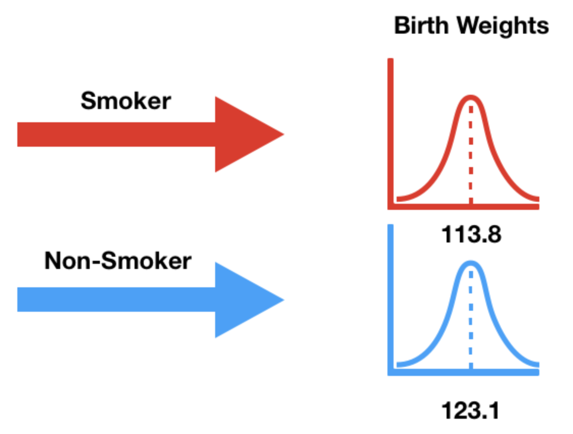
So far, our hypothesis tests have assessed a model given a single random sample.

• We flip a coin 400 times. Are the flips consistent with the coin being fair?
  • Null distribution: the coin is 50/50. This is a probability model that we can sample from.

• Do UCSD students look like a random sample of California residents?
  • Null distribution: ethnicities of California residents (e.g. 17% Asian, 3% Black, etc.). This is a probability model that we can sample from.

• Do the bill lengths of penguins on Torgersen Island look like a random sample of all bill lengths?
  • Null distribution: bill lengths of all penguins. We can sample from this distribution.

Today's lecture

Often have two random samples we wish to compare.

• Outcomes of patients assigned to control group and treatment group in a pharmaceutical study.
• Number of clicks from people who saw version A of an advertisement vs. version B.
• Pressure drops in New England Patriots footballs vs. Indianapolis Colts footballs.

Permutation testing

• Given two observed samples, are they fundamentally different, or could they have been generated by the same process?
• In a permutation test, we decide whether two fixed random samples come from the same distribution.
• Unlike in the previous hypothesis testing examples, when conducting a permutation test, you do not know what distribution generated your two samples!

Example: Birth weight and smoking 🚬

Birth weight and smoking

• Is there a significant difference in the weights of babies born to mothers who smoke, vs. non-smokers?
• We have two groups:
  • Babies whose mothers smoked during pregnancy.
  • Babies whose mothers did not smoke during pregnancy.
• In each group, the relevant attribute is the birth weight of the baby.

Let's start by loading in data.

# Kaiser dataset, 70s 
baby_fp = os.path.join('data', 'baby.csv')
baby = pd.read_csv(baby_fp)
baby.head()

	Birth Weight	Gestational Days	Maternal Age	Maternal Height	Maternal Pregnancy Weight	Maternal Smoker
0	120	284	27	62	100	False
1	113	282	33	64	135	False
2	128	279	28	64	115	True
3	108	282	23	67	125	True
4	136	286	25	62	93	False

Only the 'Birth Weight' and 'Maternal Smoker' columns are relevant.

smoking_and_birthweight = baby[['Maternal Smoker', 'Birth Weight']]
smoking_and_birthweight.head()

	Maternal Smoker	Birth Weight
0	False	120
1	False	113
2	True	128
3	True	108
4	False	136

Exploratory data analysis

How many babies are in each group?

smoking_and_birthweight.groupby('Maternal Smoker').count()

	Birth Weight
Maternal Smoker
False	715
True	459

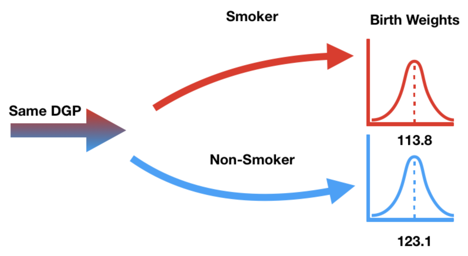
What is the average birth weight within each group?

smoking_and_birthweight.groupby('Maternal Smoker').mean()

	Birth Weight
Maternal Smoker
False	123.085315
True	113.819172

Note that 16 ounces are in 1 pound, so the above weights are ~7-8 pounds.

Visualizing birth weight distributions

• Below, we draw the distribution of birth weights, separated by mother's smoking status.
• The histograms appear to be different, but is the difference possible due to random chance or is there a significant difference in the two distributions?

title = "Birth Weight by Mother's Smoking Status"

(
    smoking_and_birthweight
    .groupby('Maternal Smoker')['Birth Weight']
    .plot(kind='hist', density=True, legend=True,
          ec='w', bins=np.arange(50, 200, 5), alpha=0.75,
          title=title)
);    

(
    smoking_and_birthweight
    .groupby('Maternal Smoker')['Birth Weight']
    .plot(kind='kde', legend=True,
          title=title)
);    

The setup

• Null hypothesis: In the population, birth weights of smokers and non-smokers have the same distribution. The difference we saw was due to random chance.
• Alternative hypothesis: In the population, babies born to smokers have lower birth weights, on average.

• Like in all of our previous hypothesis tests, we need to simulate data under the null.
• But unlike our in our previous hypothesis tests, we don't know what the null distribution is!
• Keep this thought in mind, we will revisit it momentarily.

Alternative hypothesis: birth weights come from different distributions...

• ...and babies born to mothers who smoke weigh significantly less.
• Our alternative hypothesis states that when generating birth weights, "nature" looks at whether mother smoked.
  • By "nature" here, we mean the data generating process.

Null hypothesis: birth weights come from the same distribution

• Our null hypothesis states that "smoker" / "non-smoker" labels have no relationship to birth weight.
  • In other words, the "smoker" / "non-smoker" labels may well have been assigned at random.

Choosing a test statistic

We need a test statistic that can measure how different two numerical distributions are.

(
    smoking_and_birthweight
    .groupby('Maternal Smoker')['Birth Weight']
    .plot(kind='kde', legend=True,
          title=title,
          figsize=(4, 3))
);    

Easiest solution: Difference in group means.

Difference in group means

To compute the difference between the mean birth weight of babies born to smokers and the mean birth weight of babies born to non-smokers, we can use groupby.

smoking_and_birthweight.head()

	Maternal Smoker	Birth Weight
0	False	120
1	False	113
2	True	128
3	True	108
4	False	136

means_table = smoking_and_birthweight.groupby('Maternal Smoker').mean()
means_table

	Birth Weight
Maternal Smoker
False	123.085315
True	113.819172

means_table.loc[True, 'Birth Weight'] - means_table.loc[False, 'Birth Weight']

-9.266142572024918

Note that we arbitrarily chose to compute the "smoking" mean minus the "non-smoking" mean. We could have chosen the other direction, too.

Another approach

Insteading of using .loc and manually subtracting, there is another method we can use to find the difference in group means – the diff Series/DataFrame method.

s = pd.Series([1, 2, 5, 9, 15])
s

0     1
1     2
2     5
3     9
4    15
dtype: int64

s.diff()

0    NaN
1    1.0
2    3.0
3    4.0
4    6.0
dtype: float64

means_table

	Birth Weight
Maternal Smoker
False	123.085315
True	113.819172

means_table.diff()

	Birth Weight
Maternal Smoker
False	NaN
True	-9.266143

observed_difference = means_table.diff().iloc[-1, 0]
observed_difference

-9.266142572024918

Testing through simulation

• We're almost ready to perform our hypothesis test.
  • Null hypothesis: In the population, birth weights of smokers and non-smokers have the same distribution. The difference we saw was due to random chance.
  • Alternative hypothesis: In the population, babies born to smokers have lower birth weights, on average.
  • Test statistic: Difference in group means.

• Issue: The null hypothesis doesn't say what the distribution is.
  • This is different from the coin flipping, California ethnicity, and bill length examples, because there the null hypotheses were well-defined probability models.
  • Here, we can't draw directly from the distribution!
• We have to do something a bit more clever.

Implications of the null hypothesis

• Under the null hypothesis, both groups are sampled from the same distribution.
• If this is true, then the group label – 'Maternal Smoker' – has no effect on the birth weight.
• In our dataset, we saw one assignment of True or False to each baby.

smoking_and_birthweight.head()

	Maternal Smoker	Birth Weight
0	False	120
1	False	113
2	True	128
3	True	108
4	False	136

• Under the null hypothesis, we were just as likely to see any other assignment.

Permutation tests

• In a permutation test, we generate new data by shuffling group labels.
  • In our current example, this involves randomly assigning babies to True or False, while keeping the same number of Trues and Falses as we started with.
• On each shuffle, we'll compute our test statistic (difference in group means).
• If we shuffle many times and compute our test statistic each time, we will approximate the distribution of the test statistic.
• We can them compare our observed statistic to this distribution, as in any other hypothesis test.

Shuffling

• We want to randomly shuffle the 'Maternal Smoker' column.
• The DataFrame sample method returns a random sample of rows in the DataFrame.
  • To create a permutation, either set n=df.shape[0] or frac=1.
  • By default, sample samples without replacement, which is what we want.

smoking_and_birthweight.sample(frac=1)

	Maternal Smoker	Birth Weight
803	False	116
429	False	112
557	False	170
351	True	135
1053	False	141
...	...	...
214	False	125
1013	True	103
254	True	123
459	False	130
532	True	128

1174 rows × 2 columns

Shuffling just one column

• Notice: Each time we call df.sample, both columns are shuffled together.
  • If baby 386 was assigned to False, they will still be assigned to False in the shuffled version.
• What we really want is to shuffle just one column of the DataFrame.
  • We can either shuffle the whole DataFrame and then extract one column, or extract one column and then shuffle it.
  • Shuffling just a column is quicker.
  • It doesn't matter which column we shuffle – either way, we will randomly assign babies to True or False.

A single shuffle

smoking_and_birthweight.head()

	Maternal Smoker	Birth Weight
0	False	120
1	False	113
2	True	128
3	True	108
4	False	136

Remember, it doesn't matter which column we shuffle! Here, we'll shuffle birth weights.

shuffled_weights = (
    smoking_and_birthweight['Birth Weight']
    .sample(frac=1)
    .reset_index(drop=True) # Question: What will happen if we do not reset the index?
)

shuffled_weights.head()

0     86
1    130
2    123
3    115
4    119
Name: Birth Weight, dtype: int64

original_and_shuffled = (
    smoking_and_birthweight
    .assign(**{'Shuffled Birth Weight': shuffled_weights})
)

original_and_shuffled.head(10)

	Maternal Smoker	Birth Weight	Shuffled Birth Weight
0	False	120	86
1	False	113	130
2	True	128	123
3	True	108	115
4	False	136	119
5	False	138	109
6	False	132	137
7	False	120	87
8	True	143	103
9	False	140	108

For details on how ** works, see this article.

How close are the means of the shuffled groups?

One benefit of shuffling 'Birth Weight' (instead of 'Maternal Smoker') is that grouping by 'Maternal Smoker' allows us to see all of the following information with a single call to groupby.

original_and_shuffled.groupby('Maternal Smoker').mean()

	Birth Weight	Shuffled Birth Weight
Maternal Smoker
False	123.085315	119.995804
True	113.819172	118.631808

fig, axes = plt.subplots(1, 2, figsize=(15, 5))

title = 'Birth Weights by Maternal Smoker, SHUFFLED'
original_and_shuffled.groupby('Maternal Smoker')['Shuffled Birth Weight'].plot(kind='kde', title=title, ax=axes[0])

title = 'Birth Weights by Maternal Smoker'
original_and_shuffled.groupby('Maternal Smoker')['Birth Weight'].plot(kind='kde', title=title, ax=axes[1]);

Simulation

• This was just one random shuffle.
• The question we are trying to answer is, how likely is it that a random shuffle results in a 9+ ounce difference in means?
• To answer this question, we have to repeat the process of shuffling many, many times. On each iteration, we must:
  1. Shuffle the weights.
  2. Put them in a DataFrame.
  3. Compute the test statistic (difference in group means).
  4. Store the result.

n_repetitions = 500

differences = []
for _ in range(n_repetitions):
    
    # Step 1: Shuffle the weights
    shuffled_weights = (
        smoking_and_birthweight['Birth Weight']
        .sample(frac=1)
        .reset_index(drop=True) # Be sure to reset the index! (Why?)
    )
    
    # Step 2: Put them in a DataFrame
    shuffled = (
        smoking_and_birthweight
        .assign(**{'Shuffled Birth Weight': shuffled_weights})
    )
    
    # Step 3: Compute the test statistic
    group_means = (
        shuffled
        .groupby('Maternal Smoker')
        .mean()
        .loc[:, 'Shuffled Birth Weight']
    )
    difference = group_means.diff().iloc[-1]
    
    # Step 4: Store the result
    differences.append(difference)
    
differences[:10]

[-0.03683593095357196,
 0.6106464341758482,
 -0.5090330149153601,
 -2.6160336395630566,
 -1.90058351234822,
 0.7644682115270456,
 -0.2478937184819614,
 -0.5483827719121876,
 -0.8667580785227926,
 0.5069061657297027]

We already computed the observed statistic earlier, but we compute it again below to keep all of our calculations together.

observed_difference = (
    smoking_and_birthweight
    .groupby('Maternal Smoker')['Birth Weight']
    .mean()
    .diff()
    .iloc[-1]
)

observed_difference

-9.266142572024918

Conclusion of the test

title = 'Mean Differences in Birth Weights (Smoker - Non-Smoker)'
pd.Series(differences).plot(kind='hist', density=True, ec='w', bins=10, title=title)
plt.axvline(x=observed_difference, color='red', linewidth=3);

• Under the null hypothesis, we rarely see differences as large as 9.26 ounces.
• Therefore, we reject the null hypothesis that the two groups come from the same distribution.

⚠️ Caution!

• We cannot conclude that smoking causes lower birth weight!
• This was an observational study; there may be confounding factors.
  • Maybe smokers are more likely to drink caffeine, and caffeine causes lower birth weight.
• We can't ethically perform a randomized controlled trial in this case. Why not?

Differences between categorical distributions

Example: Married vs. unmarried couples

• We will use data from a study conducted in 2010 by the National Center for Family and Marriage Research.
• The data consists of a national random sample of over 1,000 heterosexual couples who were either married or living together but unmarried.
• Each row corresponds to one person (not one couple).

couples_fp = os.path.join('data', 'married_couples.csv')
couples = pd.read_csv(couples_fp)

couples.head()

	hh_id	gender	mar_status	rel_rating	age	education	hh_income	empl_status	hh_internet
0	0	1	1	1	51	12	14	1	1
1	0	2	1	1	53	9	14	1	1
2	1	1	1	1	57	11	15	1	1
3	1	2	1	1	57	9	15	1	1
4	2	1	1	1	60	12	14	1	1

We won't use all of the columns in the DataFrame.

couples = couples[['mar_status', 'empl_status', 'gender', 'age']]
couples.head()

	mar_status	empl_status	gender	age
0	1	1	1	51
1	1	1	2	53
2	1	1	1	57
3	1	1	2	57
4	1	1	1	60

Cleaning the dataset

The numbers in the DataFrame correspond to the mappings below.

• mar_status: 1=married, 2=unmarried.
• empl_status: enumerated in the list below.
• gender: 1=male, 2=female.
• age: person's age in years.

couples.head()

	mar_status	empl_status	gender	age
0	1	1	1	51
1	1	1	2	53
2	1	1	1	57
3	1	1	2	57
4	1	1	1	60

empl = [
    'Working as paid employee',
    'Working, self-employed',
    'Not working - on a temporary layoff from a job',
    'Not working - looking for work',
    'Not working - retired',
    'Not working - disabled',
    'Not working - other'
]

couples = couples.replace({
    'mar_status': {1:'married', 2:'unmarried'},
    'gender': {1: 'M', 2: 'F'},
    'empl_status': {(k + 1): empl[k] for k in range(len(empl))}
})

couples.head()

	mar_status	empl_status	gender	age
0	married	Working as paid employee	M	51
1	married	Working as paid employee	F	53
2	married	Working as paid employee	M	57
3	married	Working as paid employee	F	57
4	married	Working as paid employee	M	60

Understanding the couples dataset

• Who is in our dataset? Mostly young people? Mostly married people? Mostly employed people?
• What is the distribution of values in each column?

# This cell shows the top 10 most common values in each column, along with their frequencies.
for col in couples:
    print(col)
    empr = couples[col].value_counts(normalize=True).to_frame().iloc[:10]
    display(empr)

mar_status

	mar_status
married	0.717602
unmarried	0.282398

empl_status

	empl_status
Working as paid employee	0.605899
Not working - other	0.103965
Working, self-employed	0.098646
Not working - looking for work	0.067698
Not working - disabled	0.056576
Not working - retired	0.050774
Not working - on a temporary layoff from a job	0.016441

gender

	gender
M	0.5
F	0.5

age

	age
53	0.037234
55	0.036750
54	0.031431
40	0.030464
44	0.029981
30	0.028046
48	0.027563
49	0.027079
52	0.027079
43	0.026596

Ages are numeric, so the previous summary was not that helpful. Let's draw a histogram.

couples['age'].plot(kind='hist', density=True, ec='w', bins=np.arange(18, 66));

Let's look at the distribution of age separately for married couples and unmarried couples.

G = couples.groupby('mar_status')
ax = G.get_group('married')['age'].rename('Married').plot(kind='hist', density=True, alpha=0.75, 
                                                          ec='w', bins=np.arange(18, 66, 2),
                                                          legend=True, title='Distribution of Ages (Married vs. Unmarried)')
G.get_group('unmarried')['age'].rename('Unmarried').plot(kind='hist', density=True, alpha=0.75, 
                                                       ec='w', bins=np.arange(18, 66, 2),
                                                       ax=ax, legend=True);

What's the difference in the two distributions? Why do you think there is a difference?

Understanding employment status in households

• Do married households more often have a stay-at-home spouse?
• Do households with unmarried couples more often have someone looking for work?
• How much does the employment status of the different households vary?

To answer these questions, let's compute the distribution of employment status conditional on household type (married vs. unmarried).

couples.head()

	mar_status	empl_status	gender	age
0	married	Working as paid employee	M	51
1	married	Working as paid employee	F	53
2	married	Working as paid employee	M	57
3	married	Working as paid employee	F	57
4	married	Working as paid employee	M	60

# Note that this is a shortcut to picking a column for values and using aggfunc='count'
empl_cnts = couples.pivot_table(index='empl_status', columns='mar_status', aggfunc='size')
empl_cnts

mar_status	married	unmarried
empl_status
Not working - disabled	72	45
Not working - looking for work	71	69
Not working - on a temporary layoff from a job	21	13
Not working - other	182	33
Not working - retired	94	11
Working as paid employee	906	347
Working, self-employed	138	66

Since there are a different number of married and unmarried couples in the dataset, we can't compare the numbers above directly. We need to convert counts to proportions, separately for married and unmarried couples.

empl_cnts.sum()

mar_status
married      1484
unmarried     584
dtype: int64

cond_distr = empl_cnts / empl_cnts.sum()
cond_distr

mar_status	married	unmarried
empl_status
Not working - disabled	0.048518	0.077055
Not working - looking for work	0.047844	0.118151
Not working - on a temporary layoff from a job	0.014151	0.022260
Not working - other	0.122642	0.056507
Not working - retired	0.063342	0.018836
Working as paid employee	0.610512	0.594178
Working, self-employed	0.092992	0.113014

Both of the columns above sum to 1.

Differences in the distributions

• Are the distributions of employment status for married people and for unmarried people who live with their partners different?
• Is this difference just due to noise?

cond_distr.plot(kind='barh', title='Distribution of Employment Status, Conditional on Household Type');

Permutation test for household composition

• Null hypothesis: In the US, the distribution of employment status among those who are married is the same as among those who are unmarried and live with their partners. The difference between the two observed samples is due to chance.

• Alternative hypothesis: In the US, the distributions of employment status of the two groups are different.

Discussion Question

What is a good test statistic in this case?

Hint: What kind of distributions are we comparing?

Total variation distance

• Whenever we need to compare two categorical distributions, we use the TVD.
  • Recall, the TVD is the sum of the absolute differences in proportions, divided by 2.
• In DSC 10, the only test statistic we ever used in permutation tests was the difference in group means/medians, but the TVD can be used in permutation tests as well.

cond_distr

mar_status	married	unmarried
empl_status
Not working - disabled	0.048518	0.077055
Not working - looking for work	0.047844	0.118151
Not working - on a temporary layoff from a job	0.014151	0.022260
Not working - other	0.122642	0.056507
Not working - retired	0.063342	0.018836
Working as paid employee	0.610512	0.594178
Working, self-employed	0.092992	0.113014

Let's first compute the observed TVD.

cond_distr.diff(axis=1).iloc[:, -1].abs().sum() / 2

0.1269754089281099

Since we'll need to calculate the TVD repeatedly, let's define a function that computes it.

couples.head()

	mar_status	empl_status	gender	age
0	married	Working as paid employee	M	51
1	married	Working as paid employee	F	53
2	married	Working as paid employee	M	57
3	married	Working as paid employee	F	57
4	married	Working as paid employee	M	60

def tvd_of_groups(df):
    cnts = df.pivot_table(index='empl_status', columns='mar_status', aggfunc='size')
    distr = cnts / cnts.sum()   # Normalized
    return distr.diff(axis=1).iloc[:, -1].abs().sum() / 2  # TVD

# Same result as above
observed_tvd = tvd_of_groups(couples)
observed_tvd

0.1269754089281099

Simulation

• Under the null hypothesis, marital status is not related to employment status.
• We can shuffle the marital status column and get an equally-likely dataset.
• On each shuffle, we will compute the TVD.
• Once we have many TVDs, we can ask, how often do we see a difference as large as our observed difference?

couples.head()

	mar_status	empl_status	gender	age
0	married	Working as paid employee	M	51
1	married	Working as paid employee	F	53
2	married	Working as paid employee	M	57
3	married	Working as paid employee	F	57
4	married	Working as paid employee	M	60

Again, let's first figure out how to perform a single shuffle. Here, we'll shuffle marital statuses.

s = couples['mar_status'].sample(frac=1).reset_index(drop=True)
s

0       unmarried
1         married
2         married
3         married
4         married
          ...    
2063      married
2064      married
2065      married
2066      married
2067    unmarried
Name: mar_status, Length: 2068, dtype: object

shuffled = couples.loc[:, ['empl_status']].assign(mar_status=s)
shuffled

	empl_status	mar_status
0	Working as paid employee	unmarried
1	Working as paid employee	married
2	Working as paid employee	married
3	Working as paid employee	married
4	Working as paid employee	married
...	...	...
2063	Working as paid employee	married
2064	Working as paid employee	married
2065	Working as paid employee	married
2066	Working as paid employee	married
2067	Working as paid employee	unmarried

2068 rows × 2 columns

tvd_of_groups(shuffled)

0.06320385481667465

Let's do this repeatedly.

N = 1000
tvds = []

for _ in range(N):
    
    s = couples['mar_status'].sample(frac=1).reset_index(drop=True)
    shuffled = couples.loc[:, ['empl_status']].assign(mar_status=s)
    
    tvds.append(tvd_of_groups(shuffled))

tvds = pd.Series(tvds)

Notice that by defining a function that computes our test statistic, our simulation code is much cleaner.

Results

pval = (tvds >= observed_tvd).sum() / N
tvds.plot(kind='hist', density=True, ec='w', bins=20, title=f'P-value: {pval}', label='Simulated TVDs')
plt.axvline(x=observed_tvd, color='red', linewidth=3, label='P-value')

perc = np.percentile(tvds, 95) # 5% significance level
plt.axvline(x=perc, color='y', linewidth=3, label='P-value cutoff')

plt.legend();

Conclusion: household composition

• We reject the null hypothesis that married/unmarried households have similar employment makeups.
• We can't say anything about why the employment makeups are different, though!

Discussion Question

In the definition of the TVD, we divide the sum of the absolute differences in proportions between the two distributions by 2.

def tvd(a, b):
    return np.sum(np.abs(a - b)) / 2

Question: If we divided by 200 instead of 2, would we still reject the null hypothesis?

An alternative investigation

• Between the two groups (married and unmarried), is there a significant difference in the proportion of people 'Not working', but either 'looking for work' or 'disabled'?
  • In other words, is there a significant difference in the proportion of people who are out of work, not by choice?
• For each group, let's compute the average number of 'Not working – looking for work' + 'Not working – disabled' individuals.

couples.head()

	mar_status	empl_status	gender	age
0	married	Working as paid employee	M	51
1	married	Working as paid employee	F	53
2	married	Working as paid employee	M	57
3	married	Working as paid employee	F	57
4	married	Working as paid employee	M	60

couples['empl_status'].value_counts()

Working as paid employee                          1253
Not working - other                                215
Working, self-employed                             204
Not working - looking for work                     140
Not working - disabled                             117
Not working - retired                              105
Not working - on a temporary layoff from a job      34
Name: empl_status, dtype: int64

The Series isin method will be helpful here.

not_work_no_choice = couples['empl_status'].isin(['Not working - looking for work', 'Not working - disabled'])
not_work_no_choice

0       False
1       False
2       False
3       False
4       False
        ...  
2063    False
2064    False
2065    False
2066    False
2067    False
Name: empl_status, Length: 2068, dtype: bool

couples['not_work_no_choice'] = not_work_no_choice.replace({True: 1, False: 0})
couples.head(12)

	mar_status	empl_status	gender	age	not_work_no_choice
0	married	Working as paid employee	M	51	0
1	married	Working as paid employee	F	53	0
2	married	Working as paid employee	M	57	0
3	married	Working as paid employee	F	57	0
4	married	Working as paid employee	M	60	0
5	married	Working as paid employee	F	57	0
6	married	Working, self-employed	M	62	0
7	married	Working as paid employee	F	59	0
8	married	Not working - other	M	53	0
9	married	Not working - retired	F	61	0
10	married	Not working - on a temporary layoff from a job	M	34	0
11	married	Not working - looking for work	F	32	1

Let's group by mar_status once again.

couples.groupby('mar_status')['not_work_no_choice'].mean()

mar_status
married      0.096361
unmarried    0.195205
Name: not_work_no_choice, dtype: float64

Notice this is not a cateogrical distribution, so we don't need to use the TVD. Instead, we can just compute the difference in group means.

obs_mean = couples.groupby('mar_status')['not_work_no_choice'].mean().diff().iloc[-1]
obs_mean

0.0988442934682273

Simulation

N = 1000
means = []

for _ in range(N):
    
    s = couples['mar_status'].sample(frac=1).reset_index(drop=True)
    shuffled = couples.loc[:, ['not_work_no_choice']].assign(mar_status=s)

    m = shuffled.groupby('mar_status')['not_work_no_choice'].mean().diff().iloc[-1]
    
    means.append(m)

means = pd.Series(means)

Results

pval = (means >= obs_mean).sum() / N
means.plot(kind='hist', density=True, ec='w', bins=20, title=f'P-value: {pval}', label='Simulated Differences in Means')
plt.axvline(x=obs_mean, color='red', linewidth=3, label='P-value')

perc = np.percentile(means, 95) # 5% significance level
plt.axvline(x=perc, color='y', linewidth=3, label='P-value cutoff')

plt.legend();

Conclusion: Household composition; not working, not by choice

Again, we reject the null hypothesis that married/unmarried households are similarly composed of those not working (not by choice) and otherwise.

Summary, next time

Summary

• Permutation tests help decide whether two samples came from the same distribution.
• In a permutation test, we simulate data under the null by shuffling either group labels or numerical features.
  • In effect, this randomly assigns individuals to groups.
• If the two distributions are numeric, we use as our test statistic the difference in group means or medians.
• If the two distributions are categorical, we use as our test statistic the total variation distance (TVD).
• Next time: How to speed up permutation tests. Revisiting missing values.