import pandas as pd
import numpy as np
import matplotlib.pyplot as plt
import seaborn as sns

plt.style.use('seaborn-white')
plt.rc('figure', dpi=100, figsize=(7, 5))
plt.rc('font', size=12)

Lecture 21 – Feature Engineering and Modeling

DSC 80, Spring 2022

Announcements

• Lab 7 is due today at 11:59PM.
• Project 4 has been released!
  • The checkpoint is due this Thursday at 11:59PM.
  • The full project is due Thursday, May 26th at 11:59PM.
  • Start early!
• 📣 Come to the DSC Town Hall, tomorrow from 3-5PM in the SDSC Auditorium.

Agenda

• Feature engineering ⚙️.
• Modeling.
• Example: Restaurant tips 🧑‍🍳.

We won't finish the galton example from the last lecture, but you should read through the end of it, as it is a nice complement to today's lecture.

Feature engineering ⚙️

The goal of feature engineering

• Feature engineering is the act of finding transformations that transform data into effective quantitative variables.

• A feature function $\phi$ (phi, pronounced "fea") is a mapping from raw data to $d$-dimensional space, i.e. $\phi: \text{raw data} \rightarrow \mathbb{R}^d$.

  • If two observations $x_i$ and $x_j$ are "similar" in the raw data space, then $\phi(x_i)$ and $\phi(x_j)$ should also be "similar."

• A "good" choice of features depends on many factors:

  • The kind of data (quantitative, ordinal, nominal),
  • The relationship(s) and association(s) being modeled,
  • The model type (e.g. linear models, decision tree models, neural networks).

Example: Predicting ratings ⭐️

• We want to build a multiple regression model that uses the features ('UID', 'AGE', 'STATE', 'HAS_BOUGHT', and 'REVIEW') below to predict 'RATING'.

• Why can't we build a model right away?

• What must we do so that we can build a model?

UID	AGE	STATE	HAS_BOUGHT	REVIEW	\		RATING
74	32	NY	True	"Meh."	|	✩✩
42	50	WA	True	"Worked out of the box..."	|	✩✩✩✩
57	16	CA	NULL	"Hella tots lit yo..."	|	✩
...	...	...	...	...	|	...
(int)	(int)	(str)	(bool)	(str)	|	(str)

• Issues: Missing values, emojis and strings instead of numbers, unrelated columns.

Uninformative features

• 'UID' was likely used to join the user information (e.g., 'AGE' and 'STATE') with some reviews dataset.
• Even though 'UID's are stored as numbers, the numerical value of a user's 'UID' won't help us predict their 'RATING'.
• If we include the 'UID' feature, our model will find whatever patterns it can between 'UID's and 'RATING's in the training (observed data).
  • This will lead to a lower training RMSE.
• However, since there is truly no relationship between 'UID' and 'RATING', this will lead to worse model performance on unseen data (bad).
• Transformation: drop 'UID'.

Dropping features

There are certain scenarios where manually dropping features might be helpful:

1. When the features do not contain information associated with the prediction task.
2. When the feature is not available at prediction time.

• The goal of building a model to predict 'RATING's is so that we can predict 'RATING's for users who haven't actually made a 'RATING's yet.
• As such, our model should only depend on features that we would know before the user makes their 'RATING'.
• For instance, if users only enter 'REVIEW's after entering 'RATING's, we shouldn't use 'REVIEW's as a feature.

Encoding ordinal features

UID	AGE	STATE	HAS_BOUGHT	REVIEW	\		RATING
74	32	NY	True	"Meh."	|	✩✩
42	50	WA	True	"Worked out of the box..."	|	✩✩✩✩
57	16	CA	NULL	"Hella tots lit yo..."	|	✩
...	...	...	...	...	|	...
(int)	(int)	(str)	(bool)	(str)	|	(str)

How do we encode the 'RATING' column, an ordinal variable, as a quantitative variable?

• Transformation: Replace "number of ✩" with "number".
  • This is an ordinal encoding, a transformation that maps ordinal values to the positive integers in a way that preserves order.
  • Example: (freshman, sophomore, junior, senior) -> (0, 1, 2, 3).
  • Important: This transformation preserves "distances" between ratings.

order_values = ['✩', '✩✩', '✩✩✩', '✩✩✩✩', '✩✩✩✩✩']
ordinal_enc = {y:x + 1 for (x, y) in enumerate(order_values)}
ordinal_enc

{'✩': 1, '✩✩': 2, '✩✩✩': 3, '✩✩✩✩': 4, '✩✩✩✩✩': 5}

ratings = pd.DataFrame().assign(RATING=['✩', '✩✩', '✩✩✩', '✩✩', '✩✩✩', '✩', '✩✩✩', '✩✩✩✩', '✩✩✩✩✩'])
ratings

	RATING
0	✩
1	✩✩
2	✩✩✩
3	✩✩
4	✩✩✩
5	✩
6	✩✩✩
7	✩✩✩✩
8	✩✩✩✩✩

ratings.replace(ordinal_enc)

	RATING
0	1
1	2
2	3
3	2
4	3
5	1
6	3
7	4
8	5

Encoding nominal features

UID	AGE	STATE	HAS_BOUGHT	REVIEW	\		RATING
74	32	NY	True	"Meh."	|	✩✩
42	50	WA	True	"Worked out of the box..."	|	✩✩✩✩
57	16	CA	NULL	"Hella tots lit yo..."	|	✩
...	...	...	...	...	|	...
(int)	(int)	(str)	(bool)	(str)	|	(str)

How do we encode the 'STATE' column, a nominal variable, as a quantitative variable?

• In other words, how do we turn 'STATE's into meaningful numbers?

• Idea: Ordinal encoding. AL -> 1, AK -> 2, ..., WY -> 50.

• ❌ An ordinal encoding is not appropriate, because 'STATE' is not an ordinal variable - Wyoming is not inherently "more" of anything than Alabama.

• Another idea: Use one binary variable per state, i.e. 'is_AL', 'is_AK', ..., 'is_WY'.

One-hot encoding

• One-hot encoding is a transformation that turns a categorical feature into several binary features.
• Suppose column 'col' has $N$ unique values, $A_1$, $A_2$, ..., $A_N$. For each unique value $A_i$, we define the following feature function:

$$\phi_i(x) = \left\{\begin{array}{ll}1 & {\rm if\ } x = A_i \\ 0 & {\rm if\ } x\neq A_i \\ \end{array}\right. $$

• Note that 1 means "yes" and 0 means "no".
• One-hot encoding is also called "dummy encoding", and $\phi(x)$ may also be referred to as an "indicator variable".

Example: One-hot encoding 'STATE'

• For each unique value of 'STATE' in our dataset, we must create a column for just that 'STATE'.

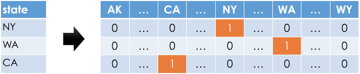
• Observations:
  • In any given row, only one of the one-hot-encoded columns will contain a 1; the rest will contain a 0.
  • Most of the values in the one-hot-encoded columns are 0, i.e. these columns are sparse.

Let's perform the one-hot encoding ourselves.

states = pd.DataFrame().assign(STATE=['NY', 'WA', 'CA', 'NY', 'OR'])
states

	STATE
0	NY
1	WA
2	CA
3	NY
4	OR

First, we need to access all unique values of 'STATE'.

unique_states = states['STATE'].unique()
unique_states

array(['NY', 'WA', 'CA', 'OR'], dtype=object)

How might we create one-hot-encoded columns manually?

states['STATE'] == unique_states[0]

0     True
1    False
2    False
3     True
4    False
Name: STATE, dtype: bool

pd.Series(states['STATE'] == unique_states[1], dtype=int)

0    0
1    1
2    0
3    0
4    0
Name: STATE, dtype: int64

def ohe_states(states_ser):
    return pd.Series(states_ser == unique_states, index=unique_states, dtype=int)

states['STATE'].apply(ohe_states)

	NY	WA	CA	OR
0	1	0	0	0
1	0	1	0	0
2	0	0	1	0
3	1	0	0	0
4	0	0	0	1

Soon, we will learn how to "automatically" perform one-hot encoding.

Quantitative scaling

The feature transformations we've discussed so far have involved converting categorical variables into quantitative variables. However, at times we'll need to transform quantitative variables into new quantitative variables.

• Standardization: $x_i \rightarrow \frac{x_i - \bar{x}}{\sigma_x}$.
• Linearization via a non-linear transformation: e.g. $\text{log}$ and $\text{sqrt}$. See Lab 8 for more.

• Discretization: Convert data into percentiles (or more generally, quantiles).

Modeling

Modeling

• Data Generating Process: The real-world phenomena that we are interested in studying.
  • Example: Every year, city employees are hired and fired, earn salaries and benefits, etc.
  • Unless we work for the city, we can't observe this process directly.

• Model: A theory about the data generating process.
  • Example: If an employee is $X$ years older than average, then they will make \$100,000 in salary.

• Fit Model: A model that is learned from a particular set of observations, i.e. training data.
  • Example: If an employee is 5 years older than average, they will make \$100,000 in salary.
  • How is this estimate determined? What makes it "good"?

Goals of modeling

• To make accurate predictions regarding unseen data drawn from the data generating process.
  • Given this dataset of past UCSD data science students' salaries, can we predict your future salary? (regression)
  • Given this dataset of emails, can we predict if this new email is spam or not? (binary classification)
  • Given this dataset of images, can we predict if this new image is of a dog, cat, or zebra? (multiclass classification)

• To make inferences about the structure of the data generating process (i.e. to understand complex phenomena).
  • Is there a linear relationship between the heights of children and the heights of their biological fathers?
  • The weights of smoking and non-smoking mothers' babies babies in my sample are different – how confident am I that this difference exists in the population?

• Of the two focuses of models, we will focus on prediction.
• In the above taxonomy, we will focus on supervised learning.

Data to models

• The modeling techniques we are most familiar with (e.g. linear regression) require:
  • Quantitative inputs.
  • Strong relationships between inputs ($X$) and outputs ($Y$).
• Often, these properties don't exist in the raw data.

• That's where feature engineering comes into play.

Example: Restaurant tips 🧑‍🍳

tips = sns.load_dataset('tips')
tips

	total_bill	tip	sex	smoker	day	time	size
0	16.99	1.01	Female	No	Sun	Dinner	2
1	10.34	1.66	Male	No	Sun	Dinner	3
2	21.01	3.50	Male	No	Sun	Dinner	3
3	23.68	3.31	Male	No	Sun	Dinner	2
4	24.59	3.61	Female	No	Sun	Dinner	4
...	...	...	...	...	...	...	...
239	29.03	5.92	Male	No	Sat	Dinner	3
240	27.18	2.00	Female	Yes	Sat	Dinner	2
241	22.67	2.00	Male	Yes	Sat	Dinner	2
242	17.82	1.75	Male	No	Sat	Dinner	2
243	18.78	3.00	Female	No	Thur	Dinner	2

244 rows × 7 columns

Predicting tips

• Goal: Given various information about a table, we want to predict the tip that a server will earn.
• Why might a server be interested in doing this?
  • To determine which tables are likely to tip the most (inference).
  • To understand the relationship between diners and tips (inference).
  • To predict earnings over the next month (prediction).

Exploratory data analysis (EDA)

• The most natural feature to look at first is 'total_bill'.
• As such, we should explore the relationship between 'total_bill' and 'tip', as well as the distributions of both columns individually.

sns.lmplot(data=tips, x='total_bill', y='tip');

fig, (ax1, ax2) = plt.subplots(1, 2, figsize=(10, 5))

sns.histplot(tips['total_bill'], kde=True, ax=ax1)
sns.histplot(tips['tip'], kde=True, ax=ax2);

Observations

'total_bill'	'tip'
Right skewed	Right skewed
Mean around \$20	Mean around \$3
Mode around \$15	Possibly bimodal?
No large bills	Large outliers?

Model #1: Constant

• Let's start simple. Suppose our model assumes every tip is given by a constant dollar amount:

$$\texttt{tip} = h^{\text{true}}$$

• Model: There is a single tip amount $h^{\text{true}}$ that all customers pay.
  • Correct? No!
  • Useful? Perhaps. An estimate of $h^{\text{true}}$, denoted by $h^*$, can allow us to predict future tips.

• The true parameter $h^{\text{true}}$ is determined by the universe (i.e. the data generating process).
  • We can't observe the parameter; we need to estimate it from the data.
  • Hence, our estimate depends on our dataset!

All models are wrong...

"...but some are useful."

"Since all models are wrong the scientist cannot obtain a "correct" one by excessive elaboration. On the contrary following William of Occam he should seek an economical description of natural phenomena. Just as the ability to devise simple but evocative models is the signature of the great scientist so overelaboration and overparameterization is often the mark of mediocrity."

"Since all models are wrong the scientist must be alert to what is importantly wrong. It is inappropriate to be concerned about mice when there are tigers abroad."

-- George Box

Estimating $h^{\text{true}}$

• There are several ways we could estimate $h^{\text{true}}$.

  • We could use domain knowledge (e.g. everyone clicks the \$1 tip option when buying coffee).

• From DSC 40A, we already know one way:

  • Choose a loss function, which measures how "good" a single prediction is.
  • Minimize empirical risk, to find the best estimate for the dataset that we have.

Empirical risk minimization

• Depending on which loss function we choose, we will end up with different $h^*$ (which are estimates of $h^{\text{true}})$.

• If we choose squared loss, then our empirical risk is mean squared error:

$$\text{MSE} = \frac{1}{n} \sum_{i = 1}^n ( y_i - h )^2 \overset{\text{calculus}}\implies h^* = \text{mean}(y)$$

• If we choose absolute loss, then our empirical risk is mean absolute error:

$$\text{MAE} = \frac{1}{n} \sum_{i = 1}^n | y_i - h | \overset{\text{algebra}}\implies h^* = \text{median}(y)$$

The mean tip

Let's suppose we choose squared loss, meaning that $h^* = \text{mean}(y)$.

mean_tip = tips['tip'].mean()
mean_tip

2.9982786885245902

Recall, minimizing MSE is the same as minimizing RMSE, however RMSE has the added benefit that it is in the same units as our data. We will compute and keep track of the RMSEs of the different models we build (as we did last lecture).

def rmse(actual, pred):
    return np.sqrt(np.mean((actual - pred) ** 2))

rmse(tips['tip'], mean_tip)

1.3807999538298958

rmse_dict = {}
rmse_dict['constant, tip'] = rmse(tips['tip'], mean_tip)

Since the mean minimizes RMSE for the constant model, it is impossible to change the mean_tip argument above to another number and yield a lower RMSE.

Model #2: Tip percentages instead of tips

• If we are going to make a constant prediction, a more natural constant to predict might be the tip percentage.

  • We know this from domain knowledge: in the US (where this dataset was collected), it is customary to tip a percentage.

• We can derive the 'pct_tip' feature ourselves using existing information: $$\texttt{pct_tip} = \frac{\texttt{tip}}{\texttt{total_bill}}$$

  • This is an example of quantitative scaling.

tips = tips.assign(pct_tip=(tips['tip'] / tips['total_bill']))
sns.histplot(tips['pct_tip'], kde=True);

The mean tip percentage

• Our model is now

$$\texttt{pct_tip} = h^{\text{true}}$$

• $h^{\text{true}}$ is the "true fixed tip percentage" that exists in the universe, that we can't observe.
• To come up with an estimate of $h^{\text{true}}$, we choose a loss function and minimize empirical risk on our observed dataset.
• Again, we'll choose squared loss, so our estimate $h^*$ will be the mean tip percentage in tips.

mean_pct_tip = tips['pct_tip'].mean()
mean_pct_tip

0.16080258172250478

• Computing the RMSE of this model is a bit more nuanced.
• To fairly compare this model to the previous model, we must still be predicting 'tip', but above we have predicted 'pct_tip'.
• Key idea:, 'pct_tip' is a multiplier that we apply to 'total_bill' to get 'tip'. That is:

$$\text{predicted tip} = \text{total bill} \cdot \text{mean pct-tip}$$

tips['total_bill'] * mean_pct_tip

0      2.732036
1      1.662699
2      3.378462
3      3.807805
4      3.954135
         ...   
239    4.668099
240    4.370614
241    3.645395
242    2.865502
243    3.019872
Name: total_bill, Length: 244, dtype: float64

rmse_dict['constant, pct_tip'] = rmse(tips['tip'], tips['total_bill'] * mean_pct_tip)
rmse_dict

{'constant, tip': 1.3807999538298958, 'constant, pct_tip': 1.146820820140744}

Constant tip vs. constant tip percentage

mean_pct_tip

0.16080258172250478

rmse_dict

{'constant, tip': 1.3807999538298958, 'constant, pct_tip': 1.146820820140744}

• A constant prediction of 16.08\% yields a lower RMSE than a constant prediction of \$3.
• However, both RMSEs are over \$1, which is relatively high compared to the mean tip amount of \\$3.
• How can we bring this RMSE down?

Model #3: Linear model

• Model: Tips are made according to a linear function:

$$\text{predicted tip} = w_0 + w_1 \cdot \text{tip}$$

• By choosing a loss function and minimizing empirical risk, we can find $w_0^*$ and $w_1^*$.

  • This process is fitting our model to the data.
  • $w_0^*$ and $w_1^*$ can be thought of as estimates of the true intercept and slope that exist in nature.

• In order to use a linear model, the data should have a linear association.

sns.lmplot(data=tips, x='total_bill', y='tip');

Fitting a linear model

Again, we will learn more about sklearn in the coming lectures.

from sklearn.linear_model import LinearRegression

lr = LinearRegression()
lr.fit(X=tips[['total_bill']], y=tips['tip'])

LinearRegression()

lr.intercept_, lr.coef_

(0.9202696135546735, array([0.10502452]))

Note that the above coefficients state that the "best way" (according to squared loss) to make tip predictions using a linear model is to assume people

• Tip ~\$0.92 up front, and
• ~10.5\% of every dollar thereafter.

preds = lr.predict(X=tips[['total_bill']])
rmse_dict['linear model'] = rmse(tips['tip'], preds)
rmse_dict

{'constant, tip': 1.3807999538298958,
 'constant, pct_tip': 1.146820820140744,
 'linear model': 1.0178504025697377}

Conclusion

• We built three models:
  • A constant model: $\text{predicted tip} = h^*$.
  • A linear model with no intercept: $\text{predicted tip} = w^* \cdot \text{total bill}$.
    • This was the model that involved tip percentage.
  • A linear model with an intercept: $\text{predicted tip} = w_0^* + w_1^* \cdot \text{total bill}$.
• As we added more features, our RMSEs decreased.
  • This was guaranteed to happen, since we were only looking at our training data.
• It is not clear that the final linear model is actually "better"; it doesn't seem to reflect reality better than the previous models.

What's next?

There's a lot of information in tips that we didn't use – 'sex', 'day', and 'time', for example. How might we encode this information?

tips

	total_bill	tip	sex	smoker	day	time	size	pct_tip
0	16.99	1.01	Female	No	Sun	Dinner	2	0.059447
1	10.34	1.66	Male	No	Sun	Dinner	3	0.160542
2	21.01	3.50	Male	No	Sun	Dinner	3	0.166587
3	23.68	3.31	Male	No	Sun	Dinner	2	0.139780
4	24.59	3.61	Female	No	Sun	Dinner	4	0.146808
...	...	...	...	...	...	...	...	...
239	29.03	5.92	Male	No	Sat	Dinner	3	0.203927
240	27.18	2.00	Female	Yes	Sat	Dinner	2	0.073584
241	22.67	2.00	Male	Yes	Sat	Dinner	2	0.088222
242	17.82	1.75	Male	No	Sat	Dinner	2	0.098204
243	18.78	3.00	Female	No	Thur	Dinner	2	0.159744

244 rows × 8 columns

Summary, next time

Summary

• To transform a categorical ordinal variable into a quantitative variable, use an ordinal encoding.
• To transform a categorical nominal variable into a quantitative variable, use one-hot encoding.
• A model is an assumption about a data generating process.
  • Models can be used for both inference and prediction.
  • All models are wrong (because they are oversimplifications of reality), but even simple models can be useful in practice.
• Next time: Finish the tips example. Start formally learning sklearn.