In [13]:
sns.lmplot(data=tips, x='total_bill', y='tip', line_kws={'color': 'red'});

import pandas as pd
import numpy as np
import matplotlib.pyplot as plt
import seaborn as sns

plt.style.use('seaborn-white')
plt.rc('figure', dpi=100, figsize=(7, 5))
plt.rc('font', size=12)
sklearn overview.sklearn.sklearn.tips = sns.load_dataset('tips')
tips
| total_bill | tip | sex | smoker | day | time | size | |
|---|---|---|---|---|---|---|---|
| 0 | 16.99 | 1.01 | Female | No | Sun | Dinner | 2 |
| 1 | 10.34 | 1.66 | Male | No | Sun | Dinner | 3 |
| 2 | 21.01 | 3.50 | Male | No | Sun | Dinner | 3 |
| 3 | 23.68 | 3.31 | Male | No | Sun | Dinner | 2 |
| 4 | 24.59 | 3.61 | Female | No | Sun | Dinner | 4 |
| ... | ... | ... | ... | ... | ... | ... | ... |
| 239 | 29.03 | 5.92 | Male | No | Sat | Dinner | 3 |
| 240 | 27.18 | 2.00 | Female | Yes | Sat | Dinner | 2 |
| 241 | 22.67 | 2.00 | Male | Yes | Sat | Dinner | 2 |
| 242 | 17.82 | 1.75 | Male | No | Sat | Dinner | 2 |
| 243 | 18.78 | 3.00 | Female | No | Thur | Dinner | 2 |
244 rows × 7 columns
The first model we looked at last class used a constant tip amount prediction for every table.
$$\text{predicted tip} = h^*$$If we use squared loss, the "best prediction is the mean of the observed tips.
mean_tip = tips['tip'].mean()
mean_tip
2.9982786885245902
def rmse(actual, pred):
    return np.sqrt(np.mean((actual - pred) ** 2))
rmse(tips['tip'], mean_tip)
1.3807999538298958
rmse_dict = {}
rmse_dict['constant, tip'] = rmse(tips['tip'], mean_tip)
The next model we created used a constant tip percentage prediction for every table.
$$\text{predicted tip percentage} = h^*$$tips = tips.assign(pct_tip=(tips['tip'] / tips['total_bill']))
tips.head()
| total_bill | tip | sex | smoker | day | time | size | pct_tip | |
|---|---|---|---|---|---|---|---|---|
| 0 | 16.99 | 1.01 | Female | No | Sun | Dinner | 2 | 0.059447 |
| 1 | 10.34 | 1.66 | Male | No | Sun | Dinner | 3 | 0.160542 |
| 2 | 21.01 | 3.50 | Male | No | Sun | Dinner | 3 | 0.166587 |
| 3 | 23.68 | 3.31 | Male | No | Sun | Dinner | 2 | 0.139780 |
| 4 | 24.59 | 3.61 | Female | No | Sun | Dinner | 4 | 0.146808 |
mean_pct_tip = tips['pct_tip'].mean()
mean_pct_tip
0.16080258172250478
'tip', but above we have predicted 'pct_tip'.'pct_tip' is a multiplier that we apply to 'total_bill' to get 'tip'. That is:tips['total_bill'] * mean_pct_tip
0      2.732036
1      1.662699
2      3.378462
3      3.807805
4      3.954135
         ...
239    4.668099
240    4.370614
241    3.645395
242    2.865502
243    3.019872
Name: total_bill, Length: 244, dtype: float64
rmse_dict['constant, pct_tip'] = rmse(tips['tip'], tips['total_bill'] * mean_pct_tip)
rmse_dict
{'constant, tip': 1.3807999538298958, 'constant, pct_tip': 1.146820820140744}
mean_pct_tip
0.16080258172250478
rmse_dict
{'constant, tip': 1.3807999538298958, 'constant, pct_tip': 1.146820820140744}
By choosing a loss function and minimizing empirical risk, we can find $w_0^*$ and $w_1^*$.
In order to use a linear model, the data should have a linear association.
sns.lmplot(data=tips, x='total_bill', y='tip', line_kws={'color': 'red'});
We'll learn more about sklearn today.
from sklearn.linear_model import LinearRegression
lr = LinearRegression()
lr.fit(X=tips[['total_bill']], y=tips['tip'])
LinearRegression()
lr.intercept_, lr.coef_
(0.9202696135546735, array([0.10502452]))
Note that the above coefficients state that the "best way" (according to squared loss) to make tip predictions using a linear model is to assume people
preds = lr.predict(X=tips[['total_bill']])
rmse_dict['simple linear model'] = rmse(tips['tip'], preds)
rmse_dict
{'constant, tip': 1.3807999538298958,
 'constant, pct_tip': 1.146820820140744,
 'simple linear model': 1.0178504025697377}
There's a lot of information in tips that we didn't use – 'sex', 'smoker', 'day', and 'time', for example. How might we encode this information?
tips.head()
| total_bill | tip | sex | smoker | day | time | size | pct_tip | |
|---|---|---|---|---|---|---|---|---|
| 0 | 16.99 | 1.01 | Female | No | Sun | Dinner | 2 | 0.059447 |
| 1 | 10.34 | 1.66 | Male | No | Sun | Dinner | 3 | 0.160542 |
| 2 | 21.01 | 3.50 | Male | No | Sun | Dinner | 3 | 0.166587 |
| 3 | 23.68 | 3.31 | Male | No | Sun | Dinner | 2 | 0.139780 |
| 4 | 24.59 | 3.61 | Female | No | Sun | Dinner | 4 | 0.146808 |
tips nominal?'day' is ordinal, but we can still use one-hot encoding.tips.head()
| total_bill | tip | sex | smoker | day | time | size | pct_tip | |
|---|---|---|---|---|---|---|---|---|
| 0 | 16.99 | 1.01 | Female | No | Sun | Dinner | 2 | 0.059447 |
| 1 | 10.34 | 1.66 | Male | No | Sun | Dinner | 3 | 0.160542 |
| 2 | 21.01 | 3.50 | Male | No | Sun | Dinner | 3 | 0.166587 |
| 3 | 23.68 | 3.31 | Male | No | Sun | Dinner | 2 | 0.139780 |
| 4 | 24.59 | 3.61 | Female | No | Sun | Dinner | 4 | 0.146808 |
categorical_cols = ['sex', 'smoker', 'day', 'time']
Let's one-hot encode the categorical columns in tips. Here's another way to do so manually:
features = tips.copy().loc[:, ['total_bill', 'size']]
for c in categorical_cols:
    for val in tips[c].unique():
        features[f'{c}={val}'] = (tips[c] == val).astype(int)
features.head()
| total_bill | size | sex=Female | sex=Male | smoker=No | smoker=Yes | day=Sun | day=Sat | day=Thur | day=Fri | time=Dinner | time=Lunch | |
|---|---|---|---|---|---|---|---|---|---|---|---|---|
| 0 | 16.99 | 2 | 1 | 0 | 1 | 0 | 1 | 0 | 0 | 0 | 1 | 0 |
| 1 | 10.34 | 3 | 0 | 1 | 1 | 0 | 1 | 0 | 0 | 0 | 1 | 0 |
| 2 | 21.01 | 3 | 0 | 1 | 1 | 0 | 1 | 0 | 0 | 0 | 1 | 0 |
| 3 | 23.68 | 2 | 0 | 1 | 1 | 0 | 1 | 0 | 0 | 0 | 1 | 0 |
| 4 | 24.59 | 4 | 1 | 0 | 1 | 0 | 1 | 0 | 0 | 0 | 1 | 0 |
Note that features has the same number of rows as tips; it just has more columns.
tips.shape
(244, 8)
features.shape
(244, 12)
Let's fit a linear model using all features in features!
lr = LinearRegression()
lr.fit(X=features, y=tips['tip'])
LinearRegression()
rmse_dict['all features'] = rmse(tips['tip'], lr.predict(X=features))
rmse_dict
{'constant, tip': 1.3807999538298958,
 'constant, pct_tip': 1.146820820140744,
 'simple linear model': 1.0178504025697377,
 'all features': 1.0051634500049156}
The RMSE of our latest model is the lowest of all linear models we've built so far (which is to be expected), but not by much. Perhaps these latest features weren't that useful.
We can visualize our latest model's predictions, too:
preds = lr.predict(X=features)

plt.figure(figsize=(10, 5))
plt.scatter(tips['total_bill'], tips['tip'], label='actual tips')
plt.scatter(tips['total_bill'], preds, label='predicted tips')
plt.xlabel('total_bill')
plt.ylabel('tip')
plt.legend();

Why don't our model's predictions lie on a straight line? 🤔
'day' and 'units sold'?sales = pd.read_csv('data/sinusoidal.csv').sort_values(by='day').reset_index(drop=True)
sales.plot(kind='scatter', x='day', y='units sold', title='Daily Sales Volume');

sns.lmplot(data=sales, x='day', y='units sold', line_kws={'color': 'red'});
sns.residplot(data=sales, x='day', y='units sold', color='orange', label='residuals');
plt.title('Units Sold vs. Day')
plt.legend();

There is a pattern in the residual plot here, which is indicative that a linear model is not the best choice.
'day' or 'units_sold' so that the resulting relationship between the two variables is roughly linear.'day' using the feature function:def transform_day(day):
return day + 5 * np.sin(2 * np.pi * day / 7)
sales['day_transformed'] = transform_day(sales['day'])
Let's draw two scatter plots:
'day_transformed' vs. 'day'.'units sold' vs. 'day'.plt.scatter(sales['day'], sales['day_transformed'], label='day_transformed')
plt.scatter(sales['day'], sales['units sold'], label='units sold')
plt.xlabel('day')
plt.legend();

While neither the orange scatter plot nor the blue scatter plot look linear, the relationship between the $y$-values in the two scatter plots is roughly linear!
Our new linear model will use 'day_transformed' as the $x$ and 'units sold' as the $y$.
sales.plot(kind='scatter', x='day_transformed', y='units sold');

sns.lmplot(data=sales, x='day_transformed', y='units sold', line_kws={'color': 'red'})
sns.residplot(data=sales, x='day_transformed', y='units sold', color='orange', label='residuals')
plt.title('Units Sold vs. Transformed Day')
plt.legend();

Now, the residual plot seems random, which is ideal!
sklearn overview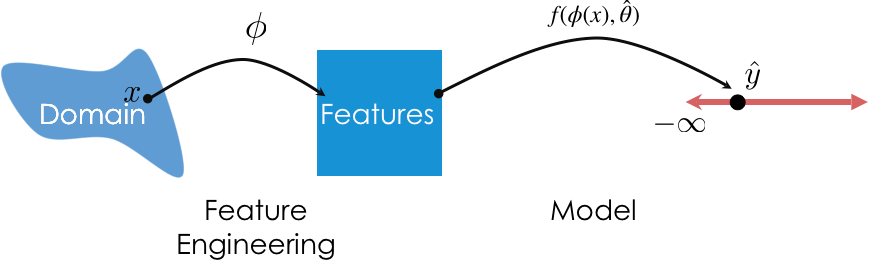
sklearn
sklearn) implements many common steps in the feature and model creation pipeline.numpy arrays, and to an extent, pandas DataFrames.preprocessing and linear_models¶For the feature creation step of the modeling pipeline, we will use sklearn's preprocessing module.

For the model creation step of the modeling pipeline, we will use sklearn's linear_model module.

sklearn¶numpy array.sklearn only looks at the values (i.e. it calls to_numpy() on input DataFrames).numpy array (never a DataFrame or Series).sklearn, are classes, not functions, meaning you need to instantiate them and call their methods.Binarizer¶The Binarizer transformer allows us to map a quantitative sequence to a sequence of 1s and 0s, depending on whether values are above or below a threshold.
| Property | Example | Description |
|---|---|---|
| Initialize with parameters | binar = Binarizer(thresh) |
set x=1 if x > thresh, else 0 |
| Transform data in a dataset | feat = binar.transform(data) |
Binarize all columns in data |
First, we need to import the relevant class from sklearn.preprocessing. (Tip: import just the relevant classes you need from sklearn.)
from sklearn.preprocessing import Binarizer
Let's try binarizing 'total_bill'. We'll say a "large" bill is one that is over \$20.
tips = sns.load_dataset('tips') # To remove the columns we "engineered" before
tips['total_bill'].head()
0    16.99
1    10.34
2    21.01
3    23.68
4    24.59
Name: total_bill, dtype: float64
First, we initialize a Binarizer object with the threshold we want.
bi = Binarizer(threshold=20)
Then, we call bi's transform method and pass it the data we'd like to transform. Note that its input and output are both 2D.
transformed_bills = bi.transform(tips[['total_bill']]) # Must pass transform a 2D array/DataFrame
transformed_bills[:5]
array([[0.],
       [0.],
       [1.],
       [1.],
       [1.]])
Cool! We can verify that it worked correctly:
((tips['total_bill'] > 20).astype(int) == transformed_bills.flatten()).all()
True
StdScaler¶StdScaler standardizes data using the mean and standard deviation of the data.Binarizer, StdScaler requires some knowledge (mean and SD) of the dataset before transforming.fit an StdScaler transformer before we can use the transform method.| Property | Example | Description |
|---|---|---|
| Initialize with parameters | stdscaler = StandardScaler() |
z-scale the data (no parameters) |
| Fit the transformer | stdscaler.fit(data) |
compute the mean and SD of data |
| Transform data in a dataset | feat = stdscaler.transform(newdata) |
z-scale newdata with mean and SD of data |
It only makes sense to standardize the already-quantitative columns of tips, so let's select just those.
tips_quant = tips[['total_bill', 'tip', 'size']]
tips_quant.head()
| total_bill | tip | size | |
|---|---|---|---|
| 0 | 16.99 | 1.01 | 2 |
| 1 | 10.34 | 1.66 | 3 |
| 2 | 21.01 | 3.50 | 3 |
| 3 | 23.68 | 3.31 | 2 |
| 4 | 24.59 | 3.61 | 4 |
Let's initialize a StandardScaler object.
from sklearn.preprocessing import StandardScaler
stdscaler = StandardScaler()
Note that the following does not work! The error message is very helpful.
stdscaler.transform(tips_quant)
---------------------------------------------------------------------------
NotFittedError                            Traceback (most recent call last)
/var/folders/pd/w73mdrsj2836_7gp0brr2q7r0000gn/T/ipykernel_14076/3962348888.py in <module>
----> 1 stdscaler.transform(tips_quant)

~/opt/anaconda3/lib/python3.9/site-packages/sklearn/preprocessing/_data.py in transform(self, X, copy)
    878             Transformed array.
    879         """
--> 880         check_is_fitted(self)
    881
    882         copy = copy if copy is not None else self.copy

~/opt/anaconda3/lib/python3.9/site-packages/sklearn/utils/validation.py in inner_f(*args, **kwargs)
     61             extra_args = len(args) - len(all_args)
     62             if extra_args <= 0:
---> 63                 return f(*args, **kwargs)
     64
     65             # extra_args > 0

~/opt/anaconda3/lib/python3.9/site-packages/sklearn/utils/validation.py in check_is_fitted(estimator, attributes, msg, all_or_any)
   1096
   1097     if not attrs:
-> 1098         raise NotFittedError(msg % {'name': type(estimator).__name__})
   1099
   1100

NotFittedError: This StandardScaler instance is not fitted yet. Call 'fit' with appropriate arguments before using this estimator.
Instead, we need to first call the fit method on stdscaler.
stdscaler.fit(tips_quant)
StandardScaler()
Now, transform will work.
# First column is 'total_bill', second column is 'tip', third column is 'size'
tips_quant_z = stdscaler.transform(tips_quant)
tips_quant_z[:5]
array([[-0.31471131, -1.43994695, -0.60019263],
       [-1.06323531, -0.96920534,  0.45338292],
       [ 0.1377799 ,  0.36335554,  0.45338292],
       [ 0.4383151 ,  0.22575414, -0.60019263],
       [ 0.5407447 ,  0.4430195 ,  1.50695847]])
We can also access the mean and variance stdscaler computed for each column:
stdscaler.mean_
array([19.78594262, 2.99827869, 2.56967213])
stdscaler.var_
array([78.92813149, 1.90660851, 0.9008835 ])
Note that we can call transform on DataFrames other than tips_quant:
stdscaler.transform(tips_quant.head(5))
array([[-0.31471131, -1.43994695, -0.60019263],
       [-1.06323531, -0.96920534,  0.45338292],
       [ 0.1377799 ,  0.36335554,  0.45338292],
       [ 0.4383151 ,  0.22575414, -0.60019263],
       [ 0.5407447 ,  0.4430195 ,  1.50695847]])
OneHotEncoder¶Let's keep just the categorical columns in tips.
tips_cat = tips[['sex', 'smoker', 'day', 'time']]
tips_cat.head()
| sex | smoker | day | time | |
|---|---|---|---|---|
| 0 | Female | No | Sun | Dinner |
| 1 | Male | No | Sun | Dinner |
| 2 | Male | No | Sun | Dinner |
| 3 | Male | No | Sun | Dinner |
| 4 | Female | No | Sun | Dinner |
Like StdScaler, we will need to fit our OneHotEncoder transformer before it can transform anything.
from sklearn.preprocessing import OneHotEncoder
ohe = OneHotEncoder()
ohe.fit(tips_cat)
OneHotEncoder()
We can look at the unique values (i.e. categories) in each column by using the categories_ attribute:
ohe.categories_
[array(['Female', 'Male'], dtype=object),
 array(['No', 'Yes'], dtype=object),
 array(['Fri', 'Sat', 'Sun', 'Thur'], dtype=object),
 array(['Dinner', 'Lunch'], dtype=object)]
ohe_features = ohe.transform(tips_cat)
ohe_features
<244x10 sparse matrix of type '<class 'numpy.float64'>'
	with 976 stored elements in Compressed Sparse Row format>
Since the resulting matrix is sparse – most of its elements are 0 – sklearn uses a more efficient representation than a regular numpy array. That's no issue, though:
ohe_features.toarray()
array([[1., 0., 1., ..., 0., 1., 0.],
       [0., 1., 1., ..., 0., 1., 0.],
       [0., 1., 1., ..., 0., 1., 0.],
       ...,
       [0., 1., 0., ..., 0., 1., 0.],
       [0., 1., 1., ..., 0., 1., 0.],
       [1., 0., 1., ..., 1., 1., 0.]])
Notice that the column names from tips_cat are no longer stored anywhere (remember, fit converts the input to a numpy array before proceeding).
We can use the get_feature_names method on ohe to access the names of the one-hot-encoded columns, though:
ohe.get_feature_names() # x0, x1, x2, and x3 correspond to column names in tips_cat
array(['x0_Female', 'x0_Male', 'x1_No', 'x1_Yes', 'x2_Fri', 'x2_Sat',
       'x2_Sun', 'x2_Thur', 'x3_Dinner', 'x3_Lunch'], dtype=object)
ohe also has an inverse_transform method, which takes a one-hot-encoded matrix and returns a categorical matrix.
ohe.inverse_transform(ohe_features[:10])
array([['Female', 'No', 'Sun', 'Dinner'],
       ['Male', 'No', 'Sun', 'Dinner'],
       ['Male', 'No', 'Sun', 'Dinner'],
       ['Male', 'No', 'Sun', 'Dinner'],
       ['Female', 'No', 'Sun', 'Dinner'],
       ['Male', 'No', 'Sun', 'Dinner'],
       ['Male', 'No', 'Sun', 'Dinner'],
       ['Male', 'No', 'Sun', 'Dinner'],
       ['Male', 'No', 'Sun', 'Dinner'],
       ['Male', 'No', 'Sun', 'Dinner']], dtype=object)
sklearn¶sklearn model classes (called "estimators") behave like transformers, in that we need to instantiate and fit them.fit is the same as "training our model".linear_model package; we will start with LinearRegression. LinearRegression class¶We've seen this a few times in lecture already, but never formally.
from sklearn.linear_model import LinearRegression
Important: From the documentation, we have
LinearRegression fits a linear model with coefficients w = (w1, …, wp) to minimize the residual sum of squares between the observed targets in the dataset, and the targets predicted by the linear approximation.
In other words, LinearRegression minimizes mean squared error by default.
Additionally, by default the fit_intercept argument is set to True.
LinearRegression?
'tip' from 'total_bill' and 'size'¶tips.head()
| total_bill | tip | sex | smoker | day | time | size | |
|---|---|---|---|---|---|---|---|
| 0 | 16.99 | 1.01 | Female | No | Sun | Dinner | 2 |
| 1 | 10.34 | 1.66 | Male | No | Sun | Dinner | 3 |
| 2 | 21.01 | 3.50 | Male | No | Sun | Dinner | 3 |
| 3 | 23.68 | 3.31 | Male | No | Sun | Dinner | 2 |
| 4 | 24.59 | 3.61 | Female | No | Sun | Dinner | 4 |
First, we instantiate and fit. By calling fit, we are saying "minimize mean squared error and find $w^*$".
lr = LinearRegression()

# Note that there are two arguments to fit – X and y!
# (It is not necessary to write X= and y=)
lr.fit(X=tips[['total_bill', 'size']], y=tips['tip'])
LinearRegression()
After fitting, the predict method is available. Note that the argument to predict can be any 2D array with two columns.
# Predicted tip from a table of 3 that spends $25
lr.predict([[25, 3]])
array([3.56457154])
# Predicted tip from a table of 14 that spends $1000 – probably not accurate!
lr.predict([[1000, 14]])
array([96.07865069])
We can access the intercepts and slopes individually. This model is of the form
$$\text{predicted tip} = w_0^* + w_1^* \cdot \text{total bill} + w_2^* \cdot \text{table size}$$so we should expect three parameters total.
lr.intercept_
0.6689447408125031
lr.coef_
array([0.09271334, 0.19259779])
If we want to compute the RMSE of our model, we need to find its predictions on every row in the training data (tips).
all_preds = lr.predict(tips[['total_bill', 'size']])
np.sqrt(np.mean((all_preds - tips['tip']) ** 2))
1.0072561271146618
It turns out that fit LinearRegression objects also have a score method:
lr.score(tips[['total_bill', 'size']], tips['tip'])
0.46786930879612587
That doesn't look like the RMSE... what is it? 🤔
Recall, all_preds contains the predicted 'tip' for every data point in tips.
tips.head()
| total_bill | tip | sex | smoker | day | time | size | |
|---|---|---|---|---|---|---|---|
| 0 | 16.99 | 1.01 | Female | No | Sun | Dinner | 2 |
| 1 | 10.34 | 1.66 | Male | No | Sun | Dinner | 3 |
| 2 | 21.01 | 3.50 | Male | No | Sun | Dinner | 3 |
| 3 | 23.68 | 3.31 | Male | No | Sun | Dinner | 2 |
| 4 | 24.59 | 3.61 | Female | No | Sun | Dinner | 4 |
all_preds[:5]
array([2.62933992, 2.20539403, 3.19464533, 3.24959215, 3.71915687])
Method 1: $R^2 = \frac{\text{var}(\text{predicted $y$ values})}{\text{var}(\text{actual $y$ values})}$
np.var(all_preds) / np.var(tips['tip'])
0.4678693087961248
Method 2: $R^2 = \left[ \text{correlation}(\text{predicted $y$ values}, \text{actual $y$ values}) \right]^2$
Note: By correlation here, we are referring to $r$.
(np.corrcoef(all_preds, tips['tip'])) ** 2
array([[1.        , 0.46786931],
       [0.46786931, 1.        ]])
Method 3: lr.score
lr.score(tips[['total_bill', 'size']], tips['tip'])
0.46786930879612587
All three methods provide the same result!
LinearRegression summary¶| Property | Example | Description |
|---|---|---|
| Initialize model parameters | lr = LinearRegression() |
Create (empty) linear regression model |
| Fit the model to the data | lr.fit(data, responses) |
Determines regression coefficients |
| Use model for prediction | lr.predict(newdata) |
Use regression line make predictions |
| Evaluate the model | lr.score(data, responses) |
Calculate the $R^2$ of the LR model |
| Access model attributes | lr.coef_ |
Access the regression coefficients |
Note: Once fit, estimators like LinearRegression are just transformers (predict <-> transform).
sklearn are used for feature engineering, while estimators in sklearn are used for models.fit.transform / predict.