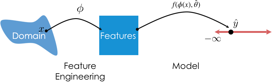
So far, we've used transformers for feature engineering and models for prediction. We can combine these steps into a single Pipeline.
import pandas as pd
import numpy as np
import matplotlib.pyplot as plt
import seaborn as sns

from sklearn.linear_model import LinearRegression

plt.style.use('seaborn-white')
plt.rc('figure', dpi=100, figsize=(7, 5))
plt.rc('font', size=12)

import warnings
warnings.simplefilter('ignore')
For fun: read this article from CBS 8 San Diego 💰🚒🚔.
Last year, the city paid \$52.93 million in overtime to the fire department. San Diego Police Department received the second highest out of any other department with \\$36.6 million.
sklearn.sklearn¶'tip' from 'total_bill' and 'size'¶tips = sns.load_dataset('tips')
tips.head()
| total_bill | tip | sex | smoker | day | time | size | |
|---|---|---|---|---|---|---|---|
| 0 | 16.99 | 1.01 | Female | No | Sun | Dinner | 2 |
| 1 | 10.34 | 1.66 | Male | No | Sun | Dinner | 3 |
| 2 | 21.01 | 3.50 | Male | No | Sun | Dinner | 3 |
| 3 | 23.68 | 3.31 | Male | No | Sun | Dinner | 2 |
| 4 | 24.59 | 3.61 | Female | No | Sun | Dinner | 4 |
First, we instantiate and fit. By calling fit, we are saying "minimize mean squared error and find $w^*$".
lr = LinearRegression()

# Note that there are two arguments to fit – X and y!
# (It is not necessary to write X= and y=)
lr.fit(X=tips[['total_bill', 'size']], y=tips['tip'])
LinearRegression()
After fitting, the predict method is available. Note that the argument to predict can be any 2D array with two columns.
# Predicted tip from a table of 3 that spends $25
lr.predict([[25, 3]])
array([3.56457154])
# Predicted tip from a table of 14 that spends $1000 – probably not accurate!
lr.predict([[1000, 14]])
array([96.07865069])
We can access the intercepts and slopes individually. This model is of the form
$$\text{predicted tip} = w_0^* + w_1^* \cdot \text{total bill} + w_2^* \cdot \text{table size}$$so we should expect three parameters total.
lr.intercept_
0.6689447408125031
lr.coef_
array([0.09271334, 0.19259779])
If we want to compute the RMSE of our model, we need to find its predictions on every row in the training data (tips).
all_preds = lr.predict(tips[['total_bill', 'size']])
np.sqrt(np.mean((all_preds - tips['tip']) ** 2))
1.007256127114662
It turns out that fit LinearRegression objects also have a score method:
lr.score(tips[['total_bill', 'size']], tips['tip'])
0.46786930879612587
That doesn't look like the RMSE... what is it? 🤔
Recall, all_preds contains the predicted 'tip' for every data point in tips.
tips.head()
| total_bill | tip | sex | smoker | day | time | size | |
|---|---|---|---|---|---|---|---|
| 0 | 16.99 | 1.01 | Female | No | Sun | Dinner | 2 |
| 1 | 10.34 | 1.66 | Male | No | Sun | Dinner | 3 |
| 2 | 21.01 | 3.50 | Male | No | Sun | Dinner | 3 |
| 3 | 23.68 | 3.31 | Male | No | Sun | Dinner | 2 |
| 4 | 24.59 | 3.61 | Female | No | Sun | Dinner | 4 |
all_preds[:5]
array([2.62933992, 2.20539403, 3.19464533, 3.24959215, 3.71915687])
Method 1: $R^2 = \frac{\text{var}(\text{predicted $y$ values})}{\text{var}(\text{actual $y$ values})}$
np.var(all_preds) / np.var(tips['tip'])
0.4678693087961252
Method 2: $R^2 = \left[ \text{correlation}(\text{predicted $y$ values}, \text{actual $y$ values}) \right]^2$
Note: By correlation here, we are referring to $r$.
(np.corrcoef(all_preds, tips['tip'])) ** 2
array([[1.        , 0.46786931],
       [0.46786931, 1.        ]])
Method 3: lr.score
lr.score(tips[['total_bill', 'size']], tips['tip'])
0.46786930879612587
All three methods provide the same result!
LinearRegression summary¶| Property | Example | Description |
|---|---|---|
| Initialize model parameters | lr = LinearRegression() |
Create (empty) linear regression model |
| Fit the model to the data | lr.fit(data, responses) |
Determines regression coefficients |
| Use model for prediction | lr.predict(newdata) |
Use regression line make predictions |
| Evaluate the model | lr.score(data, responses) |
Calculate the $R^2$ of the LR model |
| Access model attributes | lr.coef_ |
Access the regression coefficients |
Note: Once fit, estimators like LinearRegression are just transformers (predict <-> transform).
So far, we've used transformers for feature engineering and models for prediction. We can combine these steps into a single Pipeline.
Pipelines in sklearn¶Pipeline object is instantiated using a list containing transformer(s) and a model (estimator).pl = Pipeline([feat_trans1, feat_trans2, ..., mdl])
Pipeline is instantiated, you can fit all steps (transformers and model) using fit.pl.fit(data, responses)
pl.predict.Pipeline¶Pipeline, we must provide a list with zero or more transformers followed by a single model.fit methods, and all but the last must have transform methods.Pipeline with must be a list of tuples, whereLet's build a Pipeline that:
tips.tips_cat = tips[['sex', 'smoker', 'day', 'time']]
tips_cat.head()
| sex | smoker | day | time | |
|---|---|---|---|---|
| 0 | Female | No | Sun | Dinner |
| 1 | Male | No | Sun | Dinner |
| 2 | Male | No | Sun | Dinner |
| 3 | Male | No | Sun | Dinner |
| 4 | Female | No | Sun | Dinner |
from sklearn.pipeline import Pipeline
from sklearn.preprocessing import OneHotEncoder
pl = Pipeline([
    ('one-hot', OneHotEncoder()),
    ('lin-reg', LinearRegression())
])
Now that pl is instantiated, we fit it the same way we would fit the individual steps.
pl.fit(tips_cat, tips['tip'])
Pipeline(steps=[('one-hot', OneHotEncoder()), ('lin-reg', LinearRegression())])
Now, to make predictions using raw data, all we need to do is use pl.predict:
pl.predict([['Male', 'Yes', 'Sat', 'Lunch']])
array([2.58813051])
pl.predict(tips_cat.iloc[:5])
array([3.10415414, 3.27436302, 3.27436302, 3.27436302, 3.10415414])
pl performs both feature transformation and prediction with just a single call to predict!
We can access individual "steps" of a Pipeline through the named_steps attribute:
pl.named_steps
{'one-hot': OneHotEncoder(), 'lin-reg': LinearRegression()}
pl.named_steps['one-hot'].transform(tips_cat).toarray()
array([[1., 0., 1., ..., 0., 1., 0.],
       [0., 1., 1., ..., 0., 1., 0.],
       [0., 1., 1., ..., 0., 1., 0.],
       ...,
       [0., 1., 0., ..., 0., 1., 0.],
       [0., 1., 1., ..., 0., 1., 0.],
       [1., 0., 1., ..., 1., 1., 0.]])
pl.named_steps['lin-reg'].coef_
array([-0.08510444,  0.08510444, -0.04216238,  0.04216238, -0.20256076,
       -0.12962763,  0.13756057,  0.19462781,  0.25168453, -0.25168453])
Pipelines¶ColumnTransformer.ColumnTransformer using a list of tuples, where:OneHotEncoder()).ColumnTransformer is extremely useful, but it was only added to sklearn in 2018!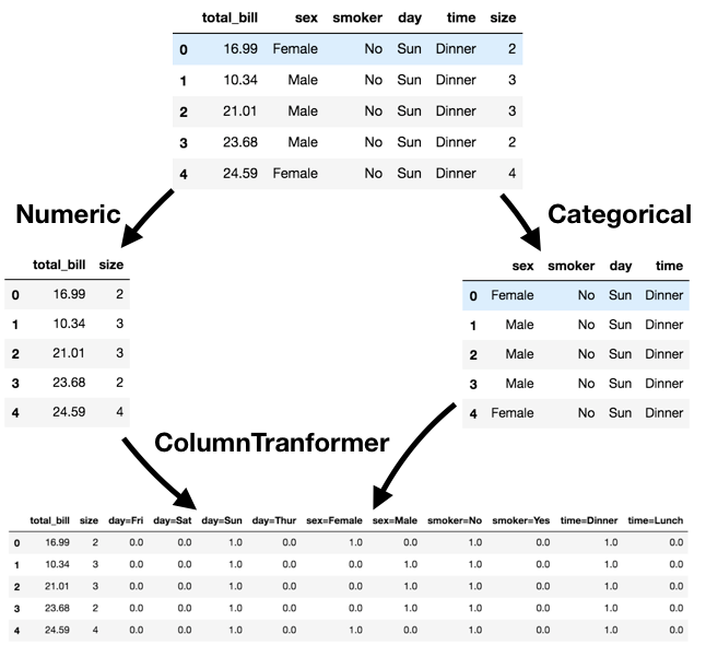
from sklearn.compose import ColumnTransformer
from sklearn.preprocessing import StandardScaler
Let's perform different transformations on the quantitative and categorical features of tips (so, we will not transform 'tip').
tips_features = tips.drop('tip', axis=1)
tips_features.head()
| total_bill | sex | smoker | day | time | size | |
|---|---|---|---|---|---|---|
| 0 | 16.99 | Female | No | Sun | Dinner | 2 |
| 1 | 10.34 | Male | No | Sun | Dinner | 3 |
| 2 | 21.01 | Male | No | Sun | Dinner | 3 |
| 3 | 23.68 | Male | No | Sun | Dinner | 2 |
| 4 | 24.59 | Female | No | Sun | Dinner | 4 |
'total_bill' and 'size'), we will apply the StandardScaler transformer.OneHotEncoder transformer.preproc = ColumnTransformer(
transformers = [
('quant', StandardScaler(), ['total_bill', 'size']),
('cat', OneHotEncoder(), ['sex', 'smoker', 'day', 'time'])
]
)
Now, let's create a Pipeline using preproc as a transformer, and fit it:
pl = Pipeline([
    ('preprocessor', preproc),
    ('lin-reg', LinearRegression())
])
pl.fit(tips_features, tips['tip'])
Pipeline(steps=[('preprocessor',
                 ColumnTransformer(transformers=[('quant', StandardScaler(),
                                                  ['total_bill', 'size']),
                                                 ('cat', OneHotEncoder(),
                                                  ['sex', 'smoker', 'day',
                                                   'time'])])),
                ('lin-reg', LinearRegression())])
Prediction is as easy as calling predict:
tips_features.head()
| total_bill | sex | smoker | day | time | size | |
|---|---|---|---|---|---|---|
| 0 | 16.99 | Female | No | Sun | Dinner | 2 |
| 1 | 10.34 | Male | No | Sun | Dinner | 3 |
| 2 | 21.01 | Male | No | Sun | Dinner | 3 |
| 3 | 23.68 | Male | No | Sun | Dinner | 2 |
| 4 | 24.59 | Female | No | Sun | Dinner | 4 |
pl.predict(tips_features.head())
array([2.73565486, 2.25086733, 3.25904369, 3.33533199, 3.80574011])
pl also has a score method, the same way a fit LinearRegression instance does:
pl.score(tips_features, tips['tip'])
0.47007812322060794
Recall, we can access the individual "steps" in pl using the named_steps attribute:
pl.named_steps['preprocessor'].transform(tips_features)
array([[-0.31471131, -0.60019263,  1.        , ...,  0.        ,
         1.        ,  0.        ],
       [-1.06323531,  0.45338292,  0.        , ...,  0.        ,
         1.        ,  0.        ],
       [ 0.1377799 ,  0.45338292,  0.        , ...,  0.        ,
         1.        ,  0.        ],
       ...,
       [ 0.3246295 , -0.60019263,  0.        , ...,  0.        ,
         1.        ,  0.        ],
       [-0.2212865 , -0.60019263,  0.        , ...,  0.        ,
         1.        ,  0.        ],
       [-0.1132289 , -0.60019263,  1.        , ...,  1.        ,
         1.        ,  0.        ]])
Note: ColumnTransformer has a remainder argument that you can use to specify what to do with columns that aren't being transfromed ('drop' or 'passthrough').
Let's collect two samples $\{(x_i, y_i)\}$ from the same data generating process.
np.random.seed(23) # For reproducibility

def sample_dgp(n=100):
    x = np.linspace(-2, 3, n)
    y = x ** 3 + (np.random.normal(0, 3, size=n))
    return x.reshape(-1, 1), y

x1, y1 = sample_dgp()
x2, y2 = sample_dgp()
For now, let's just look at Sample 1. The relationship between $x$ and $y$ is roughly cubic; that is, $y \approx x^3$ (remember, in reality, you won't get to see the DGP).
plt.scatter(x1, y1);

Let's fit three polynomial models on Sample 1:
The PolynomialFeatures transformer will be helpful here.
from sklearn.preprocessing import PolynomialFeatures
d2 = PolynomialFeatures(3)
d2.fit_transform([[1], [2], [3], [4], [5]]) # fit_transform fits and transforms the same input
array([[  1.,   1.,   1.,   1.],
       [  1.,   2.,   4.,   8.],
       [  1.,   3.,   9.,  27.],
       [  1.,   4.,  16.,  64.],
       [  1.,   5.,  25., 125.]])
degs = [1, 3, 15]

def fit_polys(x, y):
    # Create all three Pipelines
    pls = [
        Pipeline([('poly', PolynomialFeatures(d)), ('lin-reg', LinearRegression())])
        for d in degs
    ]

    # Fit all three Pipelines
    [pl.fit(x, y) for pl in pls];

    # Make all three sets of predictions
    preds = [pl.predict(x) for pl in pls]
    return preds

preds_1 = fit_polys(x1, y1)
Below, we look at our three models' predictions on Sample 1 (which they were trained on).
plt.subplots(1, 3, figsize=(15, 5), dpi=100)
plt.suptitle('Performance on Sample 1\n')

for i in range(1, 4):
    plt.subplot(1, 3, i)
    plt.scatter(x1, y1, label='actual')
    plt.plot(x1, preds_1[i-1], color='orange', label='predictions', linewidth=5)
    rmse_d = np.sqrt(np.mean((preds_1[i-1] - y1) ** 2))
    plt.title(f'Degree {degs[i-1]}, RMSE: {np.round(rmse_d, 2)}')
plt.legend(loc=(1.04, 0))
plt.show()

The degree 15 polynomial has the lowest RMSE on Sample 1.
How do things look in Sample 2?
plt.subplots(1, 3, figsize=(15, 5), dpi=100)
plt.suptitle('Performance on Sample 2\n')

for i in range(1, 4):
    plt.subplot(1, 3, i)
    plt.scatter(x2, y2, label='actual')
    plt.plot(x1, preds_1[i-1], color='orange', label='predictions', linewidth=5)
    rmse_d = np.sqrt(np.mean((preds_1[i-1] - y2) ** 2))
    plt.title(f'Degree {degs[i-1]}, RMSE: {np.round(rmse_d, 2)}')
plt.legend(loc=(1.04, 0))
plt.show()

What if we fit a degree 1, degree 3, and degree 15 polynomial on Sample 2 as well?
preds_2 = fit_polys(x2, y2)

plt.subplots(1, 3, figsize=(15, 5), dpi=100)
plt.suptitle('Models Fit on Samples 1 and 2\n')

for i in range(1, 4):
    plt.subplot(1, 3, i)
#     plt.scatter(x2, y2, label='actual')
    plt.plot(x1, preds_1[i-1], color='orange', label='Fit on Sample 1', linewidth=5)
    plt.plot(x2, preds_2[i-1], color='purple', label='Fit on Sample 2', linewidth=5)
    plt.title(f'Degree {degs[i-1]}')
plt.legend(loc=(1.04, 0))
plt.show()

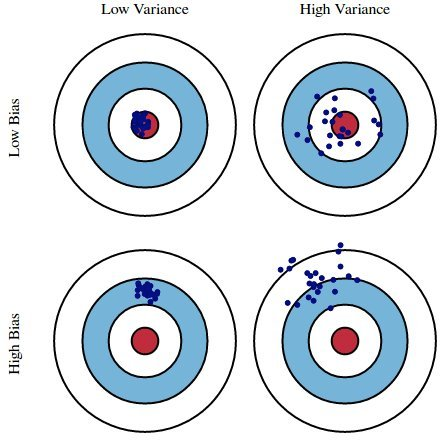
Key idea: The degree 15 polynomial seems to vary more than the degree 3 and 1 polynomials do.
The training data we have access to is a sample from the DGP. We are concerned with our model's performance across different datasets from the same DGP.
Suppose we fit a model $H$ (e.g. a degree 3 polynomial) on several different datasets from a DGP. There are three sources of error that arise:
Here, suppose
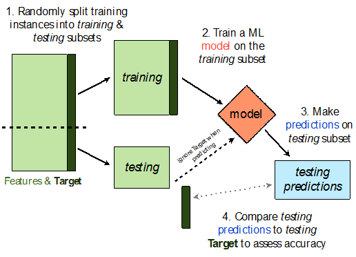
sklearn.model_selection.train_test_split implements a train-test split for us! 🙏🏼
If X is an array/DataFrame of features and y is an array/Series of responses,
X_train, X_test, y_train, y_test = train_test_split(X, y, test_size=0.25)
randomly splits the features and responses into training and test sets, such that the test set contains 0.25 of the full dataset.
from sklearn.model_selection import train_test_split
# Read the documentation!
train_test_split?
Let's perform a train/test split on our tips dataset.
X = tips.drop('tip', axis=1)
y = tips['tip']
X_train, X_test, y_train, y_test = train_test_split(X, y, test_size=0.2) # Don't have to choose 0.25
Before proceeding, let's check the sizes of X_train and X_test.
print('Rows in X_train:', X_train.shape[0])
display(X_train.head())
print('Rows in X_test:', X_test.shape[0])
display(X_test.head())
Rows in X_train: 195
| total_bill | sex | smoker | day | time | size | |
|---|---|---|---|---|---|---|
| 4 | 24.59 | Female | No | Sun | Dinner | 4 |
| 209 | 12.76 | Female | Yes | Sat | Dinner | 2 |
| 178 | 9.60 | Female | Yes | Sun | Dinner | 2 |
| 230 | 24.01 | Male | Yes | Sat | Dinner | 4 |
| 5 | 25.29 | Male | No | Sun | Dinner | 4 |
Rows in X_test: 49
| total_bill | sex | smoker | day | time | size | |
|---|---|---|---|---|---|---|
| 146 | 18.64 | Female | No | Thur | Lunch | 3 |
| 224 | 13.42 | Male | Yes | Fri | Lunch | 2 |
| 134 | 18.26 | Female | No | Thur | Lunch | 2 |
| 131 | 20.27 | Female | No | Thur | Lunch | 2 |
| 147 | 11.87 | Female | No | Thur | Lunch | 2 |
X_train.shape[0] / tips.shape[0]
0.7991803278688525
Steps:
X = tips[['total_bill', 'size']] # For this example, we'll use just the already-quantitative columns in tips
y = tips['tip']
X_train, X_test, y_train, y_test = train_test_split(X, y, test_size=0.2)
Here, we'll use a stand-alone LinearRegression model without a Pipeline, but this process would work the same if we were using a Pipeline.
lr = LinearRegression()
lr.fit(X_train, y_train)
LinearRegression()
Let's check our model's performance on the training set first.
pred_train = lr.predict(X_train)
rmse_train = np.sqrt(np.mean((pred_train - y_train) ** 2))
rmse_train
1.0142193530579229
And the test set:
pred_test = lr.predict(X_test)
rmse_test = np.sqrt(np.mean((pred_test - y_test) ** 2))
rmse_test
0.983914318376069
Since rmse_train and rmse_test are similar, it doesn't seem like our model is overfitting to the training data. If rmse_test was much larger than rmse_train, it would be evidence that our model is unable to generalize well.
Pipelines in sklearn combine one or more transformers with a single model (estimator), allowing us to perform feature engineering and prediction through a single object.