import pandas as pd
import numpy as np
import matplotlib.pyplot as plt
import seaborn as sns

# Carryover setup from last lecture
from sklearn.linear_model import LinearRegression
tips = sns.load_dataset('tips')

plt.style.use('seaborn-white')
plt.rc('figure', dpi=100, figsize=(7, 5))
plt.rc('font', size=12)

import warnings
warnings.simplefilter('ignore')

Lecture 24 – Cross-Validation

DSC 80, Spring 2022

Announcements

• Lab 8 is due today at 11:59PM.
• Project 4 is due Thursday, May 26th at 11:59PM.
  • IMPORTANT: See this post for more public tests for Question 5.
• Remaining assignments: Lab 9 and Project 5.

Agenda

• Train-test split.
• Hyperparameters.
• Cross-validation.
• Example: Decision trees 🌲.

Train-test split

Avoiding overfitting

• We won't know whether our model has overfit to our sample (training data) unless we get to see how well it performs on a new sample from the same DGP.

• Idea 💡: Split our sample into a training set and test set.

• Use only the training set to fit the model (i.e. find $w^*$).

• Use the test set to evaluate the model's error (RMSE, $R^2$).

• This is like "generating" new data from the same DGP!
  • Similar to bootstrapping (but not quite the same, because there is no resampling involved).
  • If our sample is not representative of the DGP, this method has limited effectiveness!

Train-test split 🚆

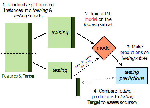
sklearn.model_selection.train_test_split implements a train-test split for us! 🙏🏼

If X is an array/DataFrame of features and y is an array/Series of responses,

X_train, X_test, y_train, y_test = train_test_split(X, y, test_size=0.25)

randomly splits the features and responses into training and test sets, such that the test set contains 0.25 of the full dataset.

from sklearn.model_selection import train_test_split

# Read the documentation!
train_test_split?

Let's perform a train/test split on our tips dataset.

X = tips.drop('tip', axis=1)
y = tips['tip']
X_train, X_test, y_train, y_test = train_test_split(X, y, test_size=0.2) # Don't have to choose 0.25

Before proceeding, let's check the sizes of X_train and X_test.

print('Rows in X_train:', X_train.shape[0])
display(X_train.head())
print('Rows in X_test:', X_test.shape[0])
display(X_test.head())

Rows in X_train: 195

	total_bill	sex	smoker	day	time	size
230	24.01	Male	Yes	Sat	Dinner	4
11	35.26	Female	No	Sun	Dinner	4
78	22.76	Male	No	Thur	Lunch	2
170	50.81	Male	Yes	Sat	Dinner	3
41	17.46	Male	No	Sun	Dinner	2

Rows in X_test: 49

	total_bill	sex	smoker	day	time	size
186	20.90	Female	Yes	Sun	Dinner	3
228	13.28	Male	No	Sat	Dinner	2
188	18.15	Female	Yes	Sun	Dinner	3
234	15.53	Male	Yes	Sat	Dinner	2
239	29.03	Male	No	Sat	Dinner	3

X_train.shape[0] / tips.shape[0]

0.7991803278688525

Example prediction pipeline

Steps:

1. Fit a model on the training set.
2. Evaluate the model on the test set.

tips.head()

	total_bill	tip	sex	smoker	day	time	size
0	16.99	1.01	Female	No	Sun	Dinner	2
1	10.34	1.66	Male	No	Sun	Dinner	3
2	21.01	3.50	Male	No	Sun	Dinner	3
3	23.68	3.31	Male	No	Sun	Dinner	2
4	24.59	3.61	Female	No	Sun	Dinner	4

X = tips[['total_bill', 'size']] # For this example, we'll use just the already-quantitative columns in tips
y = tips['tip']
X_train, X_test, y_train, y_test = train_test_split(X, y, test_size=0.2, random_state=1)

Here, we'll use a stand-alone LinearRegression model without a Pipeline, but this process would work the same if we were using a Pipeline.

lr = LinearRegression()
lr.fit(X_train, y_train)

LinearRegression()

Let's check our model's performance on the training set first.

from sklearn.metrics import mean_squared_error # built-in RMSE/MSE function

pred_train = lr.predict(X_train)
rmse_train = mean_squared_error(y_train, pred_train, squared=False)
rmse_train

0.9803205287924736

And the test set:

pred_test = lr.predict(X_test)
rmse_test = mean_squared_error(y_test, pred_test, squared=False)
rmse_test

1.138177129113125

Since rmse_train and rmse_test are similar, it doesn't seem like our model is overfitting to the training data. If rmse_test was much larger than rmse_train, it would be evidence that our model is unable to generalize well.

Hyperparameters

Example: Polynomial regression

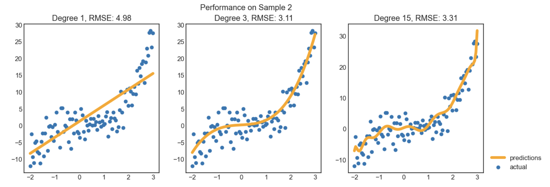
Recall, last class we looked at an example of polynomial regression.

When building these models:

• We got to choose the degree of the polynomials (i.e. we chose 1, 3, and 15).
• We didn't get to choose the exact formulas for the three polynomials – their formulas were learned from data.

Parameters vs. hyperparameters

• A parameter defines the relationship between variables in a model.

  • We learn parameters from data.

  • For instance, suppose we fit a degree 3 polynomial to data, and end up with

    $$H(x) = 1 - 2x + 13x^2 - 4x^3$$

  • 1, -2, 13, and -4 are parameters.

• A hyperparameter is a parameter that we get to choose before our model is fit to the data.
  • Think of hyperparameters as knobs 🎛 – we get to pick and tune them!
  • Polynomial degree was a hyperparameter in the previous example, and we tried three different values – 1, 3, and 15.

• Question: How do we choose the "right" hyperparameter(s)?

Training error vs. test error

• We know that a model's performance on a test set is a good estimate of its ability to generalize to unseen data.
• We want to find the hyperparameter that leads to the best test set performance.

• Idea:
  1. Come up with a list of hyperparameters to try.
  2. For each hyperparameter, train the model on the training set and compute its performance on the test set.
  3. Pick the hyperparameter with the best performance on the test set.

Training error vs. test error

• Let's try this strategy on the dataset ("Sample 1") from last class.
• We'll try to fit a polynomial model on the dataset; we'll choose the polynomial's degree from the list [1, 2, ..., 15].

sample_1 = pd.read_csv('data/sample-1.csv')
sample_1.head()

	x	y
0	-2.000000	-5.999036
1	-1.949495	-7.331676
2	-1.898990	-9.180925
3	-1.848485	-3.470179
4	-1.797980	-3.707370

plt.scatter(sample_1['x'], sample_1['y']);

First, we perform a train-test split.

X = sample_1[['x']]
y = sample_1['y']

X_train, X_test, y_train, y_test = train_test_split(X, y, random_state=100) # random_state is like np.random.seed

Now, we'll implement the logic from the previous slide.

from sklearn.pipeline import Pipeline
from sklearn.preprocessing import PolynomialFeatures

train_errs = []
test_errs = []

for d in range(1, 16):
    pl = Pipeline([('poly', PolynomialFeatures(d)), ('lin-reg', LinearRegression())])
    pl.fit(X_train, y_train)
    train_errs.append(mean_squared_error(y_train, pl.predict(X_train), squared=False))
    test_errs.append(mean_squared_error(y_test, pl.predict(X_test), squared=False))

Let's look at both the training RMSEs and test RMSEs we computed.

plt.plot(range(1, 16), train_errs, label='training RMSE')
plt.plot(range(1, 16), test_errs, label='test RMSE')
plt.xlabel('Polynomial Degree')
plt.ylabel('RMSE')
plt.legend();

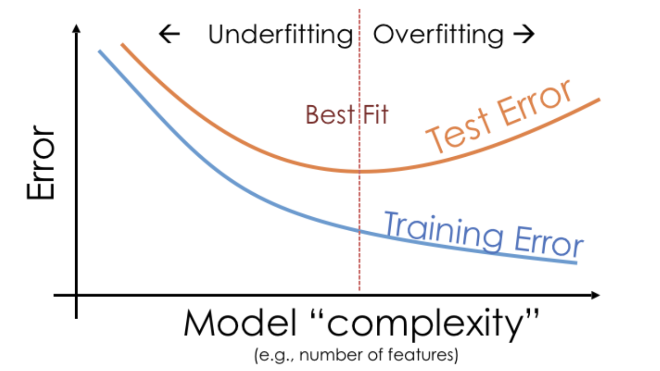
Observations:

• Training error appears to decrease as polynomial degree increases.
• Testing error appears to decrease until an "elbow", and then increases again.

Here, we'd choose a degree of 3, since that degree has the lowest test error.

Training error vs. test error

The pattern we saw in the previous example is true more generally.

We pick the hyperparameter(s) at the "valley" of test error.

Note that training error tends to underestimate test error, but it doesn't have to – i.e., it is possible for test error to be lower than training error (say, if the test set is "easier" to predict than the training set).

Conducting train-test splits

• Recall, training data is used to fit our model, and test data is used to evaluate our model.

• Question: How should we split?
  • sklearn's train_test_split splits randomly, which usually works well.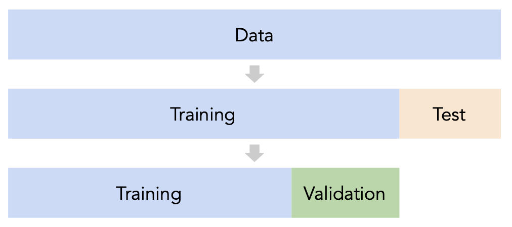
  • However, if there is some element of time in the training data (say, when predicting the future price of a stock), a better split is "past" and "future".

• Question: How large should the split be, e.g. 90%-10% vs. 75%-25%?
  • There's a tradeoff – a larger training set should lead to a "better" model, while a larger test set should lead to a better estimate of our model's ability to generalize.
  • There's no "right" choice, but we usually choose between a split between the ranges above.

But wait...

• With our current strategy, we are choosing the hyperparameter that creates the model that performs best on the test set.

• As such, we are overfitting to the test set – the best hyperparameter for the test set might not be the best hyperparameter for a totally unseen dataset!

• It seems like we need another split.

Cross-validation

A single validation set

1. Split the data into three sets: training, validation, and test.

1. For each hyperparameter choice, train the model only on the training set, and evaluate the model's performance on the validation set.

1. Find the hyperparameter with the best validation performance.

1. Retrain the final model on the training and validation sets, and report its performance on the test set.

Issue: This strategy is too dependent on the validation set, which may be small and/or not a representative sample of the data.

$k$-fold cross-validation

Instead of relying on a single validation set, we can create $k$ validation sets, where $k$ is some positive integer (5 in the following example).

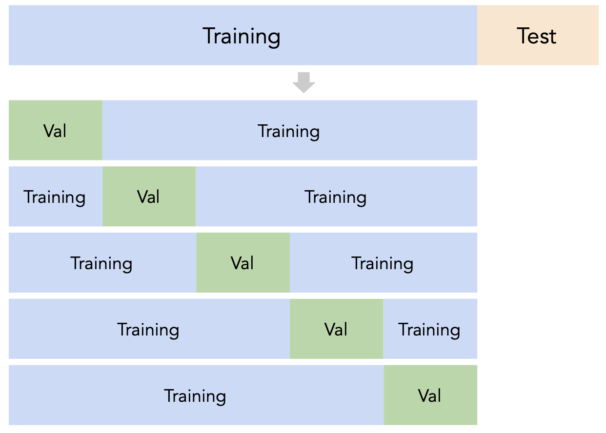
Since each data point is used for training $k-1$ times and validation once, the (averaged) validation performance should be a good metric of a model's ability to generalize to unseen data.

$k$-fold cross-validation

First, shuffle the dataset randomly and split it into $k$ disjoint groups. Then:

• For each hyperparameter:
  • For each unique group:
    • Let the unique group be the "validation set".
    • Let all other groups be the "training set".
    • Train a model using the selected hyperparameter on the training set.
    • Evaluate the model on the validation set.
  • Compute the average validation score (e.g. RMSE) for the particular hyperparameter.
• Choose the hyperparameter with the best average validation score.

Creating folds in sklearn

sklearn has a KFold class that splits data into training and validation folds.

from sklearn.model_selection import KFold

Let's use a simple dataset for illustration.

data = np.arange(10, 70, 10)
data

array([10, 20, 30, 40, 50, 60])

Let's instantiate a KFold object with $k=3$.

kfold = KFold(3, shuffle=True, random_state=1)
kfold

KFold(n_splits=3, random_state=1, shuffle=True)

Finally, let's use kfold to split data:

for train, val in kfold.split(data):
    print(f'train: {data[train]}, validation: {data[val]}')

train: [10 40 50 60], validation: [20 30]
train: [20 30 40 60], validation: [10 50]
train: [10 20 30 50], validation: [40 60]

Note that each value in data is used for validation exactly once and for training exactly twice. Also note that because we set shuffle=True the groups are not simply [10, 20], [30, 40], and [50, 60].

"Manual" $k$-fold cross-validation in sklearn

• Let's use KFold to perform $k$-fold cross validation in order to help us pick a degree for polynomial regression from the list [1, 2, ..., 15].
• We'll use $k=5$ (a common choice, and the default in sklearn).
• For the sake of example, we'll suppose sample_1 is our "training + validation data", i.e. that our test data is in some other dataset.
  • If this were not true, we'd first need to split sample_1 into train and test.

plt.scatter(sample_1['x'], sample_1['y']);

kfold = KFold(5, shuffle=True, random_state=1)

errs_df = pd.DataFrame()

for d in range(1, 16):
    errs = []
    for train, val in kfold.split(sample_1):
        # Separate the data into a training set and validation set
        data_train, data_val = sample_1.iloc[train], sample_1.iloc[val]
        
        # Fit the model on the training set
        pl = Pipeline([('poly', PolynomialFeatures(d)), ('lin-reg', LinearRegression())])
        pl.fit(data_train[['x']], data_train['y'])
        
        # Compute the model's validation error
        val_err = mean_squared_error(data_val['y'], pl.predict(data_val[['x']]), squared=False)
        errs.append(val_err)

    errs_df[f'Deg {d}'] = errs
    
errs_df.index = [f'Fold {i}' for i in range(1, 6)]

errs_df

	Deg 1	Deg 2	Deg 3	Deg 4	Deg 5	Deg 6	Deg 7	Deg 8	Deg 9	Deg 10	Deg 11	Deg 12	Deg 13	Deg 14	Deg 15
Fold 1	4.199778	3.606615	2.831147	2.828540	2.841994	2.858593	3.024709	3.065179	3.064011	3.087646	3.069269	3.035684	3.158415	3.185333	3.267513
Fold 2	6.332986	4.758864	3.359064	3.463889	4.039780	4.080516	4.156041	4.197769	4.251904	4.066354	3.876995	3.870712	3.795465	3.986883	3.487144
Fold 3	4.513414	3.091568	2.824030	2.904488	3.078070	3.201268	3.207738	3.224326	3.249295	3.317992	3.282708	3.448616	3.507821	3.561160	3.492002
Fold 4	4.554400	4.044258	3.048785	3.053034	3.148588	3.093417	3.104223	3.150751	3.322878	3.358298	3.373014	3.326871	3.529446	3.487267	4.238141
Fold 5	4.285422	3.594867	2.636512	2.676925	2.709439	3.267328	3.271033	3.268576	3.398126	3.324115	3.484460	3.498631	3.499423	3.549985	3.391811

Note that for each choice of degree (our hyperparameter), we have five RMSEs, one for each "fold" of the data.

We should choose the degree with the lowest average validation RMSE.

errs_df.mean()

Deg 1     4.777200
Deg 2     3.819234
Deg 3     2.939908
Deg 4     2.985375
Deg 5     3.163574
Deg 6     3.300225
Deg 7     3.352749
Deg 8     3.381320
Deg 9     3.457243
Deg 10    3.430881
Deg 11    3.417289
Deg 12    3.436103
Deg 13    3.498114
Deg 14    3.554126
Deg 15    3.575322
dtype: float64

errs_df.mean().idxmin()

'Deg 3'

Note that if we only performed non-$k$-fold cross-validation, we might pick a different degree:

for fold in errs_df.index:
    print(errs_df.loc[fold].idxmin())

Deg 4
Deg 3
Deg 3
Deg 3
Deg 3

"Semi-automatic" $k$-fold cross validation in sklearn

The cross_val_score function in sklearn implements a few of the previous steps in one.

cross_val_score(estimator, data, target, cv)

Specifically, it takes in:

• A Pipeline or estimator that has not already been fit
• Training data
• A value of $k$ (through the cv argument)
• (Optionally) A scoring metric

and performs $k$-fold cross-validation, returning the values of the scoring metric on each fold.

from sklearn.model_selection import cross_val_score

errs_df_auto = pd.DataFrame()

for d in range(1, 16):
    pl = Pipeline([('poly', PolynomialFeatures(d)), ('lin-reg', LinearRegression())])
    
    # The `scoring` argument is used to specify that we want to compute the RMSE; the default is R^2
    # It is called "neg" RMSE because by default sklearn likes to "maximize" scores
    errs = cross_val_score(pl, sample_1[['x']], sample_1['y'], cv=5, scoring='neg_root_mean_squared_error')
    errs_df_auto[f'Deg {d}'] = -errs # Negate to turn positive (sklearn computed negative RMSE)
    
errs_df_auto.index = [f'Fold {i}' for i in range(1, 6)]

errs_df_auto

	Deg 1	Deg 2	Deg 3	Deg 4	Deg 5	Deg 6	Deg 7	Deg 8	Deg 9	Deg 10	Deg 11	Deg 12	Deg 13	Deg 14	Deg 15
Fold 1	4.789975	12.814865	5.040947	4.927487	8.853939	13.150006	18.023855	149.574851	897.759319	718.403458	841.062760	3964.733244	55940.500810	55106.074263	202369.608764
Fold 2	3.971600	5.359234	3.186076	3.218728	3.194274	3.007987	3.077643	3.127204	3.098704	3.559998	4.260110	5.223040	4.996440	8.254853	6.843680
Fold 3	4.770176	2.557932	2.083676	2.110708	2.100757	2.013973	2.018524	1.996626	2.186183	3.946495	3.889999	3.962834	4.021369	4.912291	4.772074
Fold 4	6.134098	4.656187	2.925225	2.932392	3.030811	3.040322	3.144730	3.160528	3.310559	3.070833	2.931583	4.200841	3.894982	5.317150	3.238713
Fold 5	11.699003	11.916631	3.235882	4.372698	33.584482	51.745272	56.510688	92.223491	335.804723	1168.510898	1128.161798	8074.430848	8910.388508	9651.165907	139023.154682

errs_df_auto.mean().idxmin()

'Deg 3'

That was considerably easier! Next class, we'll look at how to streamline this procedure even more (no loop necessary).

Note: You may notice that the RMSEs in the above table, particularly in Folds 1 and 5, are much higher than they were in the manual method. Can you think of reasons why, and how we might fix this? (Hint: Go back to the "manual" method and switch shuffle to False. What do you notice?)

Summary: Generalization

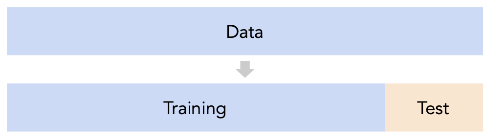
1. Split the data into two sets: training and test.

2. Use only the training data when designing, training, and tuning the model.

   • Use cross-validation to choose hyperparameters and estimate the model's ability to generalize.
   • Do not ❌ look at the test data in this step!

3. Commit to your final model and train it using the entire training set.

4. Test the data using the test data. If the performance (e.g. RMSE) is not acceptable, return to step 2.

5. Finally, train on all available data and ship the model to production! 🛳

🚨 This is the process you should always use! 🚨

Discussion Question 🤔

• Suppose you have a training dataset with 1000 rows.
• You want to decide between 20 hyperparameters for a particular model.
• To do so, you perform 10-fold cross-validation.
• How many times is the first row in the training dataset (X.iloc[0]) used for training a model?

Example: Decision trees 🌲

Decision trees can be used for both regression and classification. We will start by discussing their use in classification.

Example: Predicting diabetes

diabetes = pd.read_csv('data/diabetes.csv')
diabetes.head()

	Pregnancies	Glucose	BloodPressure	SkinThickness	Insulin	BMI	DiabetesPedigreeFunction	Age	Outcome
0	6	148	72	35	0	33.6	0.627	50	1
1	1	85	66	29	0	26.6	0.351	31	0
2	8	183	64	0	0	23.3	0.672	32	1
3	1	89	66	23	94	28.1	0.167	21	0
4	0	137	40	35	168	43.1	2.288	33	1

diabetes['Outcome'].value_counts()

0    500
1    268
Name: Outcome, dtype: int64

For illustration, we'll use 'Glucose' and 'BMI' to predict whether or not a patient has diabetes (the response variable is in the 'Outcome' column).

Building a decision tree

Let's build a decision tree and interpret the results. But first, a train-test split:

X_train, X_test, y_train, y_test = train_test_split(diabetes[['Glucose', 'BMI']], 
                                                    diabetes['Outcome'],
                                                    random_state=1)

The relevant class is DecisionTreeClassifier, from sklearn.tree.

from sklearn.tree import DecisionTreeClassifier

Note that we fit it the same way we fit earlier estimators.

_You may wonder what max_depth=2 does – more on this soon!_

dt = DecisionTreeClassifier(max_depth=2)

dt.fit(X_train, y_train)

DecisionTreeClassifier(max_depth=2)

Visualizing decision trees

Our fit decision tree is like a "flowchart", made up of a series of questions.

Class 0 (orange) is "no diabetes"; Class 1 (blue) is "diabetes".

from sklearn.tree import plot_tree

plt.figure(figsize=(10, 5))
plot_tree(dt, feature_names=X_train.columns, class_names=['no', 'yes'], 
               filled=True, rounded=True, fontsize=15, impurity=False);

• To classify a new data point, we start at the top and answer the first question (i.e. "Glucose <= 129.5").
• If the answer is "Yes", we move to the left branch, otherwise we move to the right branch.
• We repeat this process until we end up at a leaf node, at which point we predict the most common class in that node.
  • Note that each node has a value attribute, which describes the number of training individuals of each class that fell in that node.

# Note that the left node at depth 2 has a `value` of [304, 78]
y_train.loc[X_train[X_train['Glucose'] <= 129.5].index].value_counts()

0    304
1     78
Name: Outcome, dtype: int64

Evaluating classifiers

The most common evaluation metric in classification is accuracy:

$$\text{accuracy} = \frac{\text{# data points classified correctly}}{\text{# data points}}$$

(dt.predict(X_train) == y_train).mean()

0.765625

The score method of a classifier computes accuracy by default.

# Training accuracy – same number as above
dt.score(X_train, y_train)

0.765625

# Testing accuracy
dt.score(X_test, y_test)

0.7760416666666666

Some questions...

• How did sklearn decide what questions to ask?

• Can we ask more questions (i.e. build a deeper tree)?

The answers will come next class!

Summary, next time

Summary

• A model's training error tends to decrease as model complexity increases, while its test error tends to decrease, before reaching a "sweet spot" and increasing again.
• A hyperparameter is a configuration that we choose before training a model; an important task in machine learning is selecting "good" hyperparameters.
• In order to quantify a model's ability to generalize to unseen data, use $k$-fold cross-validation.
  • In particular, $k$-fold CV is used to select hyperparameters.
• Decision trees can be used for classification and regression.