import pandas as pd
import numpy as np
import matplotlib.pyplot as plt
import seaborn as sns
from matplotlib_inline.backend_inline import set_matplotlib_formats
from IPython.display import display, IFrame

# Pandas Tutor setup
%reload_ext pandas_tutor
%set_pandas_tutor_options {"maxDisplayCols": 8, "nohover": True, "projectorMode": True}

set_matplotlib_formats("svg")
sns.set_context("poster")
sns.set_style("whitegrid")
plt.rcParams["figure.figsize"] = (10, 5)
pd.set_option("display.max_rows", 8)
pd.set_option("display.max_columns", 8)
pd.set_option("display.precision", 2)

def show_paradox_slides():
    src = 'https://docs.google.com/presentation/d/e/2PACX-1vSbFSaxaYZ0NcgrgqZLvjhkjX-5MQzAITWAsEFZHnix3j1c0qN8Vd1rogTAQP7F7Nf5r-JWExnGey7h/embed?start=false'
    width = 960
    height = 569
    display(IFrame(src, width, height))

Lecture 4 – Simpson's Paradox, Joining, Transforming

DSC 80, Fall 2023

📣 Announcements 📣

• Good job going to the right lecture room!
  • Discussion in Center 115.
• Lab 2 due Monday.
• Project 1 due next Wed.

Clarification about for loops

• We've said that for loops are bad, and we should avoid them.
  • Then you had to use them a lot for Lab 1 and Project 1, what gives?
• Usually, using a for loop to iterate through individual values of a dataframe is slow.
  • Prefer to use filtering, grouping, etc.
  • But for loops are still the best way to iterate over Python values (e.g. a dictionary).
• On assignments, we won't take off points for using for loops unless explicitly stated in the question.

Review: Distributions

penguins = sns.load_dataset('penguins').dropna()

Joint distribution

When using aggfunc='count', a pivot table describes the joint distribution of two categorical variables. This is also called a contingency table.

counts = penguins.pivot_table(
    index='species', 
    columns='sex', 
    values='body_mass_g', 
    aggfunc='count', 
    fill_value=0
)
counts

sex	Female	Male
species
Adelie	73	73
Chinstrap	34	34
Gentoo	58	61

Discussion question:

Suppose we draw one penguin from penguins at random. Compute the following probabilities:

1. P(Adelie | Female)
2. P(Female | Adelie)
3. P(Male)
4. P(Chinstrap ⋂ Male)

counts

sex	Female	Male
species
Adelie	73	73
Chinstrap	34	34
Gentoo	58	61

# Compute your answers here

Simpson's paradox

Example: Grades

• Two students, Lisa and Bart, just finished freshman year. They both took a different number of classes in Fall, Winter, and Spring.

• Each quarter, Lisa had a higher GPA than Bart.

• But Bart has a higher overall GPA.

• How is this possible? 🤔

Run this cell to create DataFrames that contain each students' grades.

lisa = pd.DataFrame([[20, 46], [18, 54], [5, 20]],
    columns=['Units', 'Grade Points Earned'], 
    index=['Fall', 'Winter', 'Spring'],
)

bart = pd.DataFrame([[5, 10], [5, 13.5], [22, 81.4]],
    columns=['Units', 'Grade Points Earned'], 
    index=['Fall', 'Winter', 'Spring'],
)

Quarter-specific vs. overall GPAs

Note: The number of "grade points" earned for a course is

$$\text{number of units} \cdot \text{grade (out of 4)}$$

For instance, an A- in a 4 unit course earns $3.7 \cdot 4 = 14.8$ grade points.

lisa

	Units	Grade Points Earned
Fall	20	46
Winter	18	54
Spring	5	20

bart

	Units	Grade Points Earned
Fall	5	10.0
Winter	5	13.5
Spring	22	81.4

Lisa had a higher GPA in all three quarters:

quarterly_gpas = pd.DataFrame({
    "Lisa's Quarter GPA": lisa['Grade Points Earned'] / lisa['Units'],
    "Bart's Quarter GPA": bart['Grade Points Earned'] / bart['Units'],
})

quarterly_gpas

	Lisa's Quarter GPA	Bart's Quarter GPA
Fall	2.3	2.0
Winter	3.0	2.7
Spring	4.0	3.7

But Lisa's overall GPA was less than Bart's overall GPA:

tot = lisa.sum()
tot['Grade Points Earned'] / tot['Units']

2.7906976744186047

tot = bart.sum()
tot['Grade Points Earned'] / tot['Units']

3.278125

What happened?

(quarterly_gpas
 .assign(Lisa_units=lisa['Units'],
         Bart_units=bart['Units']) 
 .iloc[:, [0, 2, 1, 3]]
)

	Lisa's Quarter GPA	Lisa_units	Bart's Quarter GPA	Bart_units
Fall	2.3	20	2.0	5
Winter	3.0	18	2.7	5
Spring	4.0	5	3.7	22

• When Lisa and Bart both performed poorly, Lisa took more units than Bart. This brought down 📉 Lisa's overall average.

• When Lisa and Bart both performed well, Bart took more units than Annie. This brought up 📈 Bart's overall average.

Simpson's paradox

• Simpson's paradox occurs when grouped data and ungrouped data show opposing trends.

  • It is named after Edward H. Simpson, not Lisa or Bart Simpson.

• It is purely arithmetic – it is a consequence of weighted averages.

• It often happens because there is a hidden factor (i.e. a confounder) within the data that influences results.

• Question: What is the "correct" way to summarize your data? What if you had to act on these results?

Example: How Berkeley was almost sued for gender discrimination (1973)

What do you notice?

show_paradox_slides()

What happened?

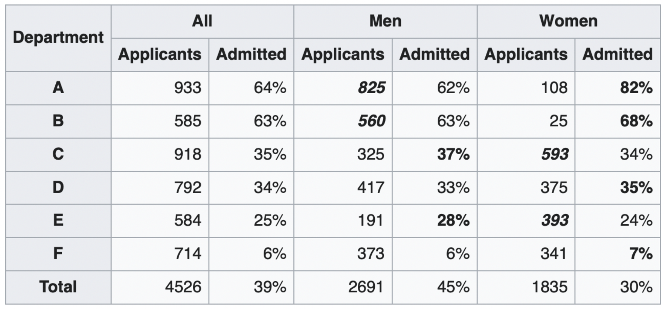
• The overall acceptance rate for women (30%) was lower than it was for men (45%).

• However, most departments (A, B, D, F) had a higher acceptance rate for women.

• Department A had a 62% acceptance rate for men and an 82% acceptance rate for women!

  • 31% of men applied to Department A.
  • 6% of women applied to Department A.

• Department F had a 6% acceptance rate for men and a 7% acceptance rate for women!

  • 14% of men applied to Department F.
  • 19% of women applied to Department F.

• Conclusion: Women tended to apply to departments with a lower acceptance rate; the data don't support the hypothesis that there was major gender discrimination against women.

Caution!

This doesn't mean that admissions are free from gender discrimination!

From Moss-Racusin et al., 2012, PNAS (cited 2600+ times):

In a randomized double-blind study (n = 127), science faculty from research-intensive universities rated the application materials of a student—who was randomly assigned either a male or female name—for a laboratory manager position. Faculty participants rated the male applicant as significantly more competent and hireable than the (identical) female applicant. These participants also selected a higher starting salary and offered more career mentoring to the male applicant. The gender of the faculty participants did not affect responses, such that female and male faculty were equally likely to exhibit bias against the female student.

But then...

From Williams and Ceci, 2015, PNAS:

Here we report five hiring experiments in which faculty evaluated hypothetical female and male applicants, using systematically varied profiles disguising identical scholarship, for assistant professorships in biology, engineering, economics, and psychology. Contrary to prevailing assumptions, men and women faculty members from all four fields preferred female applicants 2:1 over identically qualified males with matching lifestyles (single, married, divorced), with the exception of male economists, who showed no gender preference.

Do these conflict?

Not necessarily. One explanation, from William and Ceci:

Instead, past studies have used ratings of students’ hirability for a range of posts that do not include tenure-track jobs, such as managing laboratories or performing math assignments for a company. However, hiring tenure-track faculty differs from hiring lower-level staff: it entails selecting among highly accomplished candidates, all of whom have completed Ph.D.s and amassed publications and strong letters of support. Hiring bias may occur when applicants’ records are ambiguous, as was true in studies of hiring bias for lower-level staff posts, but such bias may not occur when records are clearly strong, as is the case with tenure-track hiring.

Do these conflict?

From Witteman, et al, 2019, in The Lancet:

Thus, evidence of scientists favouring women comes exclusively from hypothetical scenarios, whereas evidence of scientists favouring men comes from hypothetical scenarios and real behaviour. This might reflect academics' growing awareness of the social desirability of achieving gender balance, while real academic behaviour might not yet put such ideals into action.

Example: Restaurant reviews and phone types

• You are deciding whether to eat at Dirty Birds or The Loft.

• Suppose Yelp shows ratings aggregated by phone type (Android vs. iPhone).

Phone Type	Stars for Dirty Birds	Stars for The Loft
Android	4.24	4.0
iPhone	2.99	2.79
All	3.32	3.37

• Question: Should you choose Dirty Birds or The Loft?
• Answer: The type of phone you use likely has nothing to do with your taste in food – pick the restaurant that is rated higher overall.
• Remember, Simpson's paradox is merely a property of weighted averages!

Rule of thumb 👍

• Let $(X, Y)$ be a pair of variables of interest. Simpson's paradox happens when the association between $X$ and $Y$ reverses when we condition on $Z$, a third variable.
• If $Z$ has a causal connection to both $X$ and $Y$, we should condition on $Z$ and use deaggregated data.
• If not, we shouldn't condition on $Z$ and use the aggregated data instead.
• Berkeley gender discrimination: $X$ is gender, $Y$ is acceptance rate. $Z$ is the department.
  • $Z$ has a plausible causal effect on both $X$ and $Y$, so we should condition on $Z$.
• Yelp ratings: $X$ is the restaurant, $Y$ is the average stars. $Z$ is the phone type.
  • $Z$ doesn't plausibly cause $X$ to change, so we should not condition on $Z$.

Takeaways

Be skeptical of...

• Aggregate statistics.
• People misusing statistics to "prove" that discrimination doesn't exist.
• Drawing conclusions from individual publications ($p$-hacking, publication bias, narrow focus, etc.).
• Everything!

We need to apply domain knowledge and human judgement calls to decide what to do when Simpson's paradox is present.

Really?

To handle Simpson's paradox with rigor, we need some ideas from causal inference which we don't have time to cover in DSC 80. This video has a good example of how to approach Simpson's paradox using a minimal amount of causal inference, if you're curious (not required for DSC 80).

IFrame('https://www.youtube-nocookie.com/embed/zeuW1Z2EtLs?si=l2Dl7P-5RCq3ODpo',
       width=560, height=315)

Further reading

• Gender Bias in Admission Statistics?
  • Contains a great visualization, but seems to be paywalled now.
• What is Simpson's Paradox?
• Understanding Simpson's Paradox: Requires more statistics background, gives rigorous understanding of when to use aggregated vs. unaggregated data.

Merging

Motivating Example: Name categories

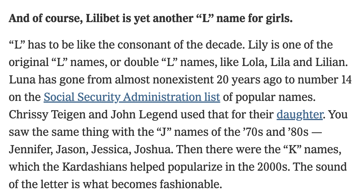
NYT article about baby names (https://archive.is/NpORG) says that certain categories of names are becoming more popular. For example:

1. Forbidden names like Lucifer, Lilith, Kali, and Danger.
2. Evangelical names like Amen, Savior, Canaan, and Creed.
3. Mythological names
4. etc.

And also, baby boomer names are becoming less popular.

Let's see if we can verify these claims using data!

baby = pd.read_csv('data/baby.csv')
baby

	Name	Sex	Count	Year
0	Liam	M	20456	2022
1	Noah	M	18621	2022
2	Olivia	F	16573	2022
3	Oliver	M	15076	2022
...	...	...	...	...
2085154	Worthy	M	5	1880
2085155	Wright	M	5	1880
2085156	York	M	5	1880
2085157	Zachariah	M	5	1880

2085158 rows × 4 columns

nyt = pd.read_csv('data/nyt_names.csv')
nyt

	nyt_name	category
0	Lucifer	forbidden
1	Lilith	forbidden
2	Danger	forbidden
3	Amen	evangelical
...	...	...
19	Amethyst	mineral
20	Venus	celestial
21	Celestia	celestial
22	Skye	celestial

23 rows × 2 columns

Joining

• We want to link rows together whenever the names match up.
• This is a join (SQL term), i.e. a merge (pandas term).
• A join is appropriate when we have two sources of information about the same individuals that is linked by a common column(s).
• The common column(s) are called the join key.

Let's demonstrate on a small subset of baby and nyt.

nyt_small = nyt.iloc[[11, 12, 14]].reset_index(drop=True)

names_to_keep = ['Julius', 'Karen', 'Noah']
baby_small = (baby
 .query("Year == 2020 and Name in @names_to_keep")
 .reset_index(drop=True)
)

nyt_small

	nyt_name	category
0	Karen	boomer
1	Julius	mythology
2	Freya	mythology

baby_small

	Name	Sex	Count	Year
0	Noah	M	18407	2020
1	Julius	M	966	2020
2	Karen	F	330	2020
3	Noah	F	306	2020
4	Karen	M	6	2020

Let's do a join!

%%pt
baby_small.merge(nyt_small, left_on='Name', right_on='nyt_name')

The merge method

• The merge DataFrame method joins two tables by columns or indexes.

  • "Merge" is just the pandas word for "join".

• When using the merge method, the DataFrame before .merge is the "left" DataFrame, and the DataFrame passed into .merge is the "right" DataFrame.

  • In baby_small.merge(nyt_small), baby_small is considered the "left" DataFrame and nyt_small is the "right" DataFrame; the columns from the left DataFrame appear to the left of the columns from right DataFrame.

• By default:

  • If join keys are not specified, all shared columns between the two DataFrames are used.
  • The "type" of join performed is an inner join.

Join types: inner joins

• Note that 'Noah' and 'Freya' do not appear in the merged DataFrame.
• This is because there is:
  • no 'Noah' in the right DataFrame, and
  • no 'Freya' in the left DataFrame.
• The default type of join that merge performs is an inner join, which keeps the intersection of the join keys.

Different join types

We can change the type of join performed by changing the how argument in merge. Let's experiment!

%%pt
# Note the NaNs!
baby_small.merge(nyt_small, left_on='Name', right_on='nyt_name', how='left')

%%pt
baby_small.merge(nyt_small, left_on='Name', right_on='nyt_name', how='right')

%%pt
baby_small.merge(nyt_small, left_on='Name', right_on='nyt_name', how='outer')

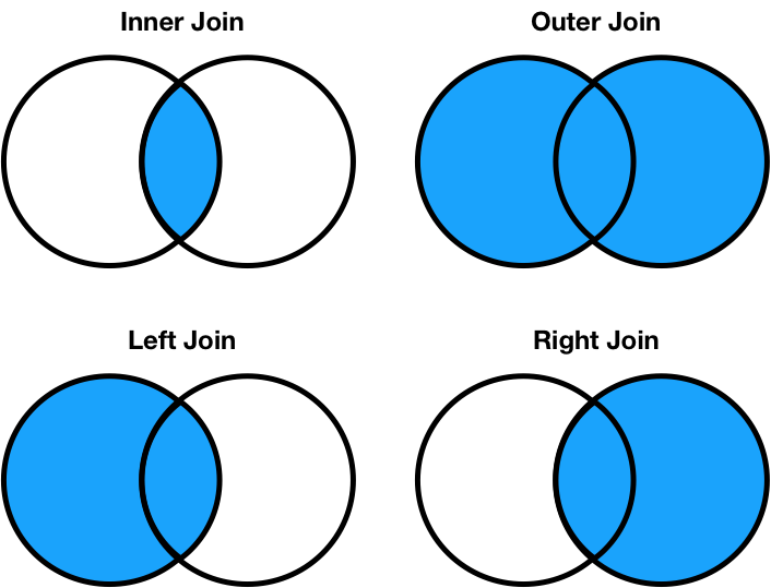
Different join types handle mismatches differently

There are four types of joins.

• Inner: keep only matching keys (intersection).
• Outer: keeps all keys in both DataFrames (union).
• Left: keep all keys in the left DataFrame, whether or not they are in the right DataFrame.
• Right: keep all keys in the right DataFrame, whether or not they are in the left DataFrame.
  • Note that a.merge(b, how='left') contains the same information as b.merge(a, how='right'), just in a different order.

Notes on the merge method

• .merge is flexible, you can merge using a combination of columns, or the index of the dataframe.
• If the two dataframes have the same column names, pandas will add _x and _y to the duplicated column names to avoid having columns with the same name (change with the suffixes argument).
• There is, in fact, a .join method, but it's actually a wrapper around .merge with fewer options.

Many-to-one & many-to-many joins

One-to-one joins

• So far in this lecture, the joins we have worked with are called one-to-one joins.
• Neither the left DataFrame nor the right DataFrame contained any duplicates in the join key.
• What if there are duplicated join keys, in one or both of the DataFrames we are merging?

# Run this cell to set up the next example.

profs = pd.DataFrame(
[['Sam', 'UCB', 5],
 ['Sam', 'UCSD', 5],
 ['Janine', 'UCSD', 8],
 ['Marina', 'UIC', 7],
 ['Justin', 'OSU', 5],
 ['Soohyun', 'UCSD', 2],
 ['Suraj', 'UCB', 2]],
    columns=['Name', 'School', 'Years']
)

schools = pd.DataFrame({
    'Abr': ['UCSD', 'UCLA', 'UCB', 'UIC'],
    'Full': ['University of California San Diego', 'University of California, Los Angeles', 'University of California, Berkeley', 'University of Illinois Chicago']
})

programs = pd.DataFrame({
    'uni': ['UCSD', 'UCSD', 'UCSD', 'UCB', 'OSU', 'OSU'],
    'dept': ['Math', 'HDSI', 'COGS', 'CS', 'Math', 'CS'],
    'grad_students': [205, 54, 281, 439, 304, 193]
})

Many-to-one joins

• Many-to-one joins are joins where one of the DataFrames contains duplicate values in the join key.
• The resulting DataFrame will preserve those duplicate entries as appropriate.

profs

	Name	School	Years
0	Sam	UCB	5
1	Sam	UCSD	5
2	Janine	UCSD	8
3	Marina	UIC	7
4	Justin	OSU	5
5	Soohyun	UCSD	2
6	Suraj	UCB	2

schools

	Abr	Full
0	UCSD	University of California San Diego
1	UCLA	University of California, Los Angeles
2	UCB	University of California, Berkeley
3	UIC	University of Illinois Chicago

Note that when merging profs and schools, the information from schools is duplicated.

• 'University of California, San Diego' appears three times.
• 'University of California, Berkeley' appears twice.

# Why is a left merge most appropriate here?
profs.merge(schools, left_on='School', right_on='Abr', how='left')

	Name	School	Years	Abr	Full
0	Sam	UCB	5	UCB	University of California, Berkeley
1	Sam	UCSD	5	UCSD	University of California San Diego
2	Janine	UCSD	8	UCSD	University of California San Diego
3	Marina	UIC	7	UIC	University of Illinois Chicago
4	Justin	OSU	5	NaN	NaN
5	Soohyun	UCSD	2	UCSD	University of California San Diego
6	Suraj	UCB	2	UCB	University of California, Berkeley

Many-to-many joins

Many-to-many joins are joins where both DataFrames have duplicate values in the join key.

profs

	Name	School	Years
0	Sam	UCB	5
1	Sam	UCSD	5
2	Janine	UCSD	8
3	Marina	UIC	7
4	Justin	OSU	5
5	Soohyun	UCSD	2
6	Suraj	UCB	2

programs

	uni	dept	grad_students
0	UCSD	Math	205
1	UCSD	HDSI	54
2	UCSD	COGS	281
3	UCB	CS	439
4	OSU	Math	304
5	OSU	CS	193

Before running the following cell, try predicting the number of rows in the output.

%%pt

profs.merge(programs, left_on='School', right_on='uni')

• merge stitched together every UCSD row in profs with every UCSD row in programs.
• Since there were 3 UCSD rows in profs and 3 in programs, there are $3 \cdot 3 = 9$ UCSD rows in the output. The same applies for all other schools.

Returning back to our original question

Let's find the popularity of baby name categories over time.

cate_counts = (
    baby
    .merge(nyt, left_on='Name', right_on='nyt_name')
    .groupby(['category', 'Year'])
    ['Count']
    .sum()
    .reset_index()
)
cate_counts

	category	Year	Count
0	boomer	1880	292
1	boomer	1881	298
2	boomer	1882	326
3	boomer	1883	322
...	...	...	...
658	mythology	2019	3330
659	mythology	2020	3516
660	mythology	2021	3895
661	mythology	2022	4049

662 rows × 3 columns

# We'll talk about plotting code soon!
import plotly.express as px
fig = px.line(cate_counts, x='Year', y='Count',
              facet_col='category', facet_col_wrap=3,
              facet_row_spacing=0.15,
              width=600, height=400)
fig.update_yaxes(matches=None, showticklabels=False)

Transforming

baby

	Name	Sex	Count	Year
0	Liam	M	20456	2022
1	Noah	M	18621	2022
2	Olivia	F	16573	2022
3	Oliver	M	15076	2022
...	...	...	...	...
2085154	Worthy	M	5	1880
2085155	Wright	M	5	1880
2085156	York	M	5	1880
2085157	Zachariah	M	5	1880

2085158 rows × 4 columns

Transforming values

The most flexible method is apply: takes in a function that receives a single value as input, returns a single value.

def number_of_vowels(string):
    return sum(c in 'aeiou' for c in string.lower())

baby['Name'].apply(number_of_vowels)

0          2
1          2
2          4
3          3
          ..
2085154    1
2085155    1
2085156    1
2085157    4
Name: Name, Length: 2085158, dtype: int64

# Builtin functions work
baby['Name'].apply(len)

0          4
1          4
2          6
3          6
          ..
2085154    6
2085155    6
2085156    4
2085157    9
Name: Name, Length: 2085158, dtype: int64

Looking at "L" names

def first_letter(string):
    return string[0]

(baby
 .assign(first=baby['Name'].apply(first_letter))
 .query('first == "L"')
 .groupby('Year')
 ['Count']
 .sum()
 .plot()
)

<AxesSubplot:xlabel='Year'>

The Price of .apply

Actually, .apply runs really slowly!

%%timeit
baby['Name'].apply(first_letter)

151 ms ± 622 µs per loop (mean ± std. dev. of 7 runs, 10 loops each)

%%timeit
res = []
for name in baby['Name']:
    res.append(name[0])

176 ms ± 1.22 ms per loop (mean ± std. dev. of 7 runs, 10 loops each)

Internally, .apply actually just runs a for loop.

• So for arthimetic operations, definitely prefer working on Series objects directly!

The Price of .apply

%%timeit
baby['Year'] // 10 * 10

4.87 ms ± 38.1 µs per loop (mean ± std. dev. of 7 runs, 100 loops each)

%%timeit
baby['Year'].apply(lambda y: y // 10 * 10)

453 ms ± 3.43 ms per loop (mean ± std. dev. of 7 runs, 1 loop each)

100x slower!

The .str accessor

For string operations, pandas provides a convenient str accessor.

# Equivalent to:
# baby['Name'].apply(first_letter)
baby['Name'].str[0]

0          L
1          N
2          O
3          O
          ..
2085154    W
2085155    W
2085156    Y
2085157    Z
Name: Name, Length: 2085158, dtype: object

baby['Name'].str.len()

0          4
1          4
2          6
3          6
          ..
2085154    6
2085155    6
2085156    4
2085157    9
Name: Name, Length: 2085158, dtype: int64

• Very convenient, but runs even slower than .apply!
• Even though it's slow, we use .str anyway because it makes life easier.

Other Data Representations

• In DSC 80, we work with dataframes in pandas.
  • When we say pandas DataFrame, we're talking about the pandas API for its DataFrame objects.
  • When we say "dataframe", we're referring to a general way to represent data (rows, columns, labels for both rows and columns)
• Of course, many other way to work with data tables! R has a dataframe, SQL databases, spreadsheets, even matrices from linear algebra.
  • When you learn SQL in DSC 100, you'll find many similaries (e.g. slicing columns, filtering rows, grouping, joining, etc.)
  • Relational algebra captures common data operations between many data table systems.
• Why use dataframes over something else?

Dataframes vs. Spreadsheets

• Dataframes gives us a data lineage: the code records down data changes. Not so in spreadsheets!
• Using a general-purpose programming language gives us the ability to handle much larger datasets, and we can using distributed computing systems to handle massive datasets.

Dataframes vs. Matrices

\begin{split} \begin{aligned} \mathbf{X} = \begin{bmatrix} 1 & 0 \\ 0 & 4 \\ 0 & 0 \\ \end{bmatrix} \end{aligned} \end{split}

• Matrices are mathematical objects. Can only hold numbers, but have many useful properties (see the entire branch of linear algebra).
• Often, we process data from a dataframe into matrix format for machine learning models. Will see this process later in DSC 80.

Dataframes vs. Relations

• Relations are the data representation for relational database systems (e.g. MySQL, PostgreSQL, etc.)
• Will learn all about these in DSC 100.
• Database systems are much better than dataframes at storing many data tables and handling concurrency (many people reading and writing data at the same time).
• Common workflow: load a subset of data in from a database system into pandas, then make plot.
• Or: load and clean data in pandas, then store in database system for others to use.

Takeaways

• Neither CS nor Statistics can tell us how to automatically resolve Simpson's paradox! Domain knowledge is important.
• We've covered main dataframe manipulations: subsetting, aggregating, joining, and transforming.
• Next time: applying what we know to real-world, messy data!