from dsc80_utils import *

# The dataset is built into plotly (and seaborn)!
# We shuffle here so that the head of the DataFrame contains rows where smoker is Yes and smoker is No,
# purely for illustration purposes (it doesn't change any of the math).
np.random.seed(1)
tips = px.data.tips().sample(frac=1).reset_index(drop=True)

def rmse(actual, pred):
    return np.sqrt(np.mean((actual - pred) ** 2))

Lecture 14 – Feature Engineering, Pipelines

DSC 80, Fall 2023

📣 Announcements 📣

• Project 4 out, due next Friday, Dec 1.
  • No project checkpoint due because of Thanksgiving, so everyone gets full credit for the checkpoint!
  • But start early! Historically, the last two questions of the project take up about 75% of the project time.
• Lab 8 out, due Nov 27.
• No lecture / discussion / OH on Thurs or Fri. Happy Thanksgiving! 🦃

📆 Agenda

• Review: Linear models for restaurant tips
• Feature engineering
• Scikit-learn pipelines

🙋🙋🏽‍♀️ Slido

https://app.sli.do/event/2LZSnXWNpGPiuVnCZMa5J8

Review: Linear Models for Restaurant tips 🧑‍🍳

tips

	total_bill	tip	sex	smoker	day	time	size
0	3.07	1.00	Female	Yes	Sat	Dinner	1
1	18.78	3.00	Female	No	Thur	Dinner	2
2	26.59	3.41	Male	Yes	Sat	Dinner	3
...	...	...	...	...	...	...	...
241	17.47	3.50	Female	No	Thur	Lunch	2
242	10.07	1.25	Male	No	Sat	Dinner	2
243	16.93	3.07	Female	No	Sat	Dinner	3

244 rows × 7 columns

from sklearn.linear_model import LinearRegression

mean_tip = tips['tip'].mean()

model = LinearRegression()
model.fit(X=tips[['total_bill']], y=tips['tip'])

model_two = LinearRegression()
model_two.fit(X=tips[['total_bill', 'size']], y=tips['tip'])

LinearRegression()

rmse_dict = {}
rmse_dict['constant tip amount'] = rmse(tips['tip'], mean_tip)

all_preds = model.predict(tips[['total_bill']])
rmse_dict['one feature: total bill'] = rmse(tips['tip'], all_preds)

rmse_dict['two features'] = rmse(
    tips['tip'], model_two.predict(tips[['total_bill', 'size']])
)
rmse_dict

{'constant tip amount': 1.3807999538298956,
 'one feature: total bill': 1.0178504025697377,
 'two features': 1.0072561271146618}

Calculating $R^2$

all_preds contains model_two's predicted 'tip' for every row in tips.

pred = tips.assign(predicted=model_two.predict(tips[['total_bill', 'size']]))
pred

	total_bill	tip	sex	smoker	day	time	size	predicted
0	3.07	1.00	Female	Yes	Sat	Dinner	1	1.15
1	18.78	3.00	Female	No	Thur	Dinner	2	2.80
2	26.59	3.41	Male	Yes	Sat	Dinner	3	3.71
...	...	...	...	...	...	...	...	...
241	17.47	3.50	Female	No	Thur	Lunch	2	2.67
242	10.07	1.25	Male	No	Sat	Dinner	2	1.99
243	16.93	3.07	Female	No	Sat	Dinner	3	2.82

244 rows × 8 columns

Method 1: $R^2 = \frac{\text{var}(\text{predicted $y$ values})}{\text{var}(\text{actual $y$ values})}$

np.var(pred['predicted']) / np.var(pred['tip'])

0.4678693087961255

Method 2: $R^2 = \left[ \text{correlation}(\text{predicted $y$ values}, \text{actual $y$ values}) \right]^2$

Note: By correlation here, we are referring to $r$, the same correlation coefficient you saw in DSC 10.

# There was a typo here last lecture, the correct code is:
(np.corrcoef(pred['predicted'], pred['tip'])) ** 2

array([[1.  , 0.47],
       [0.47, 1.  ]])

Method 3: LinearRegression.score

model_two.score(tips[['total_bill', 'size']], tips['tip'])

0.46786930879612565

All three methods provide the same result!

What's next?

tips.head()

	total_bill	tip	sex	smoker	day	time	size
0	3.07	1.00	Female	Yes	Sat	Dinner	1
1	18.78	3.00	Female	No	Thur	Dinner	2
2	26.59	3.41	Male	Yes	Sat	Dinner	3
3	14.26	2.50	Male	No	Thur	Lunch	2
4	21.16	3.00	Male	No	Thur	Lunch	2

• So far, in our journey to predict 'tip', we've only used the existing numerical features in our dataset, 'total_bill' and 'size'.

• There's a lot of information in tips that we didn't use – 'sex', 'smoker', 'day', and 'time', for example. We can't use these features in their current form, because they're non-numeric.

• How do we use categorical features in a regression model?

Feature engineering ⚙️

The goal of feature engineering

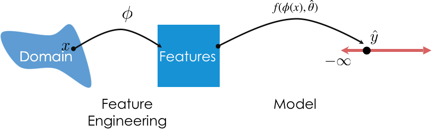
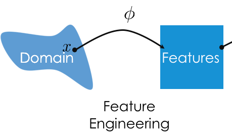
• Feature engineering is the act of finding transformations that transform data into effective quantitative variables.

• A feature function $\phi$ (phi, pronounced "fea") is a mapping from raw data to $d$-dimensional space, i.e. $\phi: \text{raw data} \rightarrow \mathbb{R}^d$.

  • If two observations $x_i$ and $x_j$ are "similar" in the raw data space, then $\phi(x_i)$ and $\phi(x_j)$ should also be "similar."

• A "good" choice of features depends on many factors:

  • The kind of data (quantitative, ordinal, nominal).
  • The relationship(s) and association(s) being modeled.
  • The model type (e.g. linear models, decision tree models, neural networks).

One hot encoding

• One hot encoding is a transformation that turns a categorical feature into several binary features.

• Suppose column 'col' has $N$ unique values, $A_1$, $A_2$, ..., $A_N$. For each unique value $A_i$, we define the following feature function:

$$\phi_i(x) = \left\{\begin{array}{ll}1 & {\rm if\ } x = A_i \\ 0 & {\rm if\ } x\neq A_i \\ \end{array}\right. $$

• Note that 1 means "yes" and 0 means "no".

• One hot encoding is also called "dummy encoding", and $\phi(x)$ may also be referred to as an "indicator variable".

Example: One hot encoding 'smoker'

For each unique value of 'smoker' in our dataset, we must create a column for just that 'smoker'. (Remember, 'smoker' is 'Yes' when the table was in the smoking section of the restaurant and 'No' otherwise.)

tips.head()

	total_bill	tip	sex	smoker	day	time	size
0	3.07	1.00	Female	Yes	Sat	Dinner	1
1	18.78	3.00	Female	No	Thur	Dinner	2
2	26.59	3.41	Male	Yes	Sat	Dinner	3
3	14.26	2.50	Male	No	Thur	Lunch	2
4	21.16	3.00	Male	No	Thur	Lunch	2

tips['smoker'].value_counts()

No     151
Yes     93
Name: smoker, dtype: int64

(tips['smoker'] == 'Yes').astype(int).head()

0    1
1    0
2    1
3    0
4    0
Name: smoker, dtype: int64

for val in tips['smoker'].unique():
    tips[f'smoker == {val}'] = (tips['smoker'] == val).astype(int)

tips.head()

	total_bill	tip	sex	smoker	...	time	size	smoker == Yes	smoker == No
0	3.07	1.00	Female	Yes	...	Dinner	1	1	0
1	18.78	3.00	Female	No	...	Dinner	2	0	1
2	26.59	3.41	Male	Yes	...	Dinner	3	1	0
3	14.26	2.50	Male	No	...	Lunch	2	0	1
4	21.16	3.00	Male	No	...	Lunch	2	0	1

5 rows × 9 columns

Model #4: Multiple linear regression using total bill, table size, and smoker status

Now that we've converted 'smoker' to a numerical variable, we can use it as input in a regression model. Here's the model we'll try to fit:

$$\text{predicted tip} = w_0 + w_1 \cdot \text{total bill} + w_2 \cdot \text{table size} + w_3 \cdot \text{smoker == Yes}$$

Subtlety: There's no need to use both 'smoker == No' and 'smoker == Yes'. If we know the value of one, we already know the value of the other. We can use either one.

model_three = LinearRegression()
model_three.fit(tips[['total_bill', 'size', 'smoker == Yes']], tips['tip'])

LinearRegression()

The following cell gives us our $w^*$s:

model_three.intercept_, model_three.coef_

(0.7090155167346053, array([ 0.09,  0.18, -0.08]))

Thus, our trained linear model to predict tips given total bills, table sizes, and smoker status (yes or no) is:

$$\text{predicted tip} = 0.709 + 0.094 \cdot \text{total bill} + 0.180 \cdot \text{table size} - 0.083 \cdot \text{smoker == Yes}$$

Visualizing Model #4

Our new fit model is:

$$\text{predicted tip} = 0.709 + 0.094 \cdot \text{total bill} + 0.180 \cdot \text{table size} - 0.083 \cdot \text{smoker == Yes}$$

To visualize our data and linear model, we'd need 4 dimensions:

• One for total bill
• One for table size
• One for 'smoker == Yes'.
• One for tip.

Humans can't visualize in 4D, but there may be a solution. We know that 'smoker == Yes' only has two possible values, 1 or 0, so let's look at those cases separately.

Case 1: 'smoker == Yes' is 1, meaning that the table was in the smoking section.

$$\begin{align*} \text{predicted tip} &= 0.709 + 0.094 \cdot \text{total bill} + 0.180 \cdot \text{table size} - 0.083 \cdot 1 \\ &= 0.626 + 0.094 \cdot \text{total bill} + 0.180 \cdot \text{table size} \end{align*}$$

Case 2: 'smoker == Yes' is 0, meaning that the table was not in the smoking section.

$$\begin{align*} \text{predicted tip} &= 0.709 + 0.094 \cdot \text{total bill} + 0.180 \cdot \text{table size} - 0.083 \cdot 0 \\ &= 0.709 + 0.094 \cdot \text{total bill} + 0.180 \cdot \text{table size} \end{align*}$$

Key idea: These are two parallel planes in 3D, with different $z$-intercepts!

Note that the two planes are very close to one another – you'll have to zoom in to see the difference.

XX, YY = np.mgrid[0:50:2, 0:8:1]
Z_0 = model_three.intercept_ + model_three.coef_[0] * XX + model_three.coef_[1] * YY + model_three.coef_[2] * 0
Z_1 = model_three.intercept_ + model_three.coef_[0] * XX + model_three.coef_[1] * YY + model_three.coef_[2] * 1
plane_0 = go.Surface(x=XX, y=YY, z=Z_0, colorscale='Greens')
plane_1 = go.Surface(x=XX, y=YY, z=Z_1, colorscale='Purples')

fig = go.Figure(data=[plane_0, plane_1])

tips_0 = tips[tips['smoker'] == 'No']
tips_1 = tips[tips['smoker'] == 'Yes']

fig.add_trace(go.Scatter3d(x=tips_0['total_bill'], 
                           y=tips_0['size'], 
                           z=tips_0['tip'], mode='markers', marker = {'color': 'green'}))

fig.add_trace(go.Scatter3d(x=tips_1['total_bill'], 
                           y=tips_1['size'], 
                           z=tips_1['tip'], mode='markers', marker = {'color': 'purple'}))

fig.update_layout(scene = dict(
    xaxis_title='Total Bill',
    yaxis_title='Table Size',
    zaxis_title='Tip'),
  title='Tip vs. Total Bill and Table Size (Green = Non-Smoking Section, Purple = Smoking Section)',
    width=1000, height=800,
    showlegend=False)

If we want to visualize in 2D, we need to pick a single feature to place on the $x$-axis.

fig = go.Figure()
fig.add_trace(go.Scatter(x=tips['total_bill'], y=tips['tip'], 
                         mode='markers', name='Original Data'))
fig.add_trace(go.Scatter(x=tips['total_bill'], y=model_three.predict(tips[['total_bill', 'size', 'smoker == Yes']]), 
                         mode='markers', name='Predicted Tips using Total Bill, <br>Table Size, and Smoker Status'))

fig.update_layout(showlegend=True, title='Tip vs. Total Bill',
                  xaxis_title='Total Bill', yaxis_title='Tip')

Despite being a linear model, why doesn't this model look like a straight line?

🙋🙋🏽‍♀️ Questions?

https://app.sli.do/event/2LZSnXWNpGPiuVnCZMa5J8

Comparing Model #4 to earlier models

rmse_dict['three features'] = rmse(tips['tip'], 
                                   model_three.predict(tips[['total_bill', 'size', 'smoker == Yes']]))
rmse_dict

{'constant tip amount': 1.3807999538298956,
 'one feature: total bill': 1.0178504025697377,
 'two features': 1.0072561271146618,
 'three features': 1.0064899786822126}

Adding 'smoker == Yes' decreased the training RMSE of our model, but barely.

Reflection

tips.head()

	total_bill	tip	sex	smoker	...	time	size	smoker == Yes	smoker == No
0	3.07	1.00	Female	Yes	...	Dinner	1	1	0
1	18.78	3.00	Female	No	...	Dinner	2	0	1
2	26.59	3.41	Male	Yes	...	Dinner	3	1	0
3	14.26	2.50	Male	No	...	Lunch	2	0	1
4	21.16	3.00	Male	No	...	Lunch	2	0	1

5 rows × 9 columns

• We've one hot encoded 'smoker', but it required a for-loop.

• Is there an easy way to one hot encode all four categorical columns – 'sex', 'smoker', 'day', and 'time' – all at once, without using a for-loop?

• Yes, using sklearn.preprocessing's OneHotEncoder. More on this soon!

Example: Predicting ratings ⭐️

Example: Predicting ratings ⭐️

UID	AGE	STATE	HAS_BOUGHT	REVIEW	\
74	32	NY	True	"Meh."	|	✩✩
42	50	WA	True	"Worked out of the box..."	|	✩✩✩✩
57	16	CA	NULL	"Hella tots lit yo..."	|	✩
...	...	...	...	...	|	...
(int)	(int)	(str)	(bool)	(str)	|	(str)

• We want to build a multiple regression model that predicts 'RATING' using the above features.

• Why can't we build a model right away? What must we do so that we can build a model?

• Some issues: Missing values, emojis and strings instead of numbers, unrelated columns.

Uninformative features

• 'UID' was likely used to join the user information (e.g., 'AGE' and 'STATE') with some reviews dataset.
• Even though 'UID's are stored as numbers, the numerical value of a user's 'UID' won't help us predict their 'RATING'.
• If we include the 'UID' feature, our model will find whatever patterns it can between 'UID's and 'RATING's in the training (observed data).
  • This will lead to a lower training RMSE.
• However, since there is truly no relationship between 'UID' and 'RATING', this will lead to worse model performance on unseen data (bad).
• Transformation: drop 'UID'.

Dropping features

There are certain scenarios where manually dropping features might be helpful:

1. When the features do not contain information associated with the prediction task.
2. When the feature is not available at prediction time.

• The goal of building a model to predict 'RATING's is so that we can predict 'RATING's for users who haven't actually made a 'RATING's yet.
• As such, our model should only depend on features that we would know before the user makes their 'RATING'.
• For instance, if users only enter 'REVIEW's after entering 'RATING's, we shouldn't use 'REVIEW's as a feature.

Encoding ordinal features

UID	AGE	STATE	HAS_BOUGHT	REVIEW	\
74	32	NY	True	"Meh."	|	✩✩
42	50	WA	True	"Worked out of the box..."	|	✩✩✩✩
57	16	CA	NULL	"Hella tots lit yo..."	|	✩
...	...	...	...	...	|	...
(int)	(int)	(str)	(bool)	(str)	|	(str)

How do we encode the 'RATING' column, an ordinal variable, as a quantitative variable?

• Transformation: Replace "number of ✩" with "number".
  • This is an ordinal encoding, a transformation that maps ordinal values to the positive integers in a way that preserves order.
  • Example: (freshman, sophomore, junior, senior) -> (0, 1, 2, 3).
  • Important: This transformation preserves "distances" between ratings.

ordinal_enc = {
    '✩': 1,
    '✩✩': 2,
    '✩✩✩': 3,
    '✩✩✩✩': 4,
    '✩✩✩✩✩': 5,
}
ordinal_enc

{'✩': 1, '✩✩': 2, '✩✩✩': 3, '✩✩✩✩': 4, '✩✩✩✩✩': 5}

ratings = pd.DataFrame().assign(RATING=['✩', '✩✩', '✩✩✩', '✩✩', '✩✩✩', '✩', '✩✩✩', '✩✩✩✩', '✩✩✩✩✩'])
ratings

	RATING
0	✩
1	✩✩
2	✩✩✩
...	...
6	✩✩✩
7	✩✩✩✩
8	✩✩✩✩✩

9 rows × 1 columns

ratings.replace(ordinal_enc)

	RATING
0	1
1	2
2	3
...	...
6	3
7	4
8	5

9 rows × 1 columns

Encoding nominal features

UID	AGE	STATE	HAS_BOUGHT	REVIEW	\
74	32	NY	True	"Meh."	|	✩✩
42	50	WA	True	"Worked out of the box..."	|	✩✩✩✩
57	16	CA	NULL	"Hella tots lit yo..."	|	✩
...	...	...	...	...	|	...
(int)	(int)	(str)	(bool)	(str)	|	(str)

How do we encode the 'STATE' column, a nominal variable, as a quantitative variable? In other words, how do we turn 'STATE's into meaningful numbers?

• Question: Why can't we use an ordinal encoding, e.g. NY -> 0, WA -> 1?

• Answer: There is no inherent ordering to states, e.g. WA is not inherently "more" of anything than NY.

• We've already seen the correct strategy: one hot encoding.

Example: Horsepower 🚗

The following dataset, built into the seaborn plotting library, contains various information about (older) cars.

mpg = sns.load_dataset('mpg').dropna()
mpg.head()

	mpg	cylinders	displacement	horsepower	...	acceleration	model_year	origin	name
0	18.0	8	307.0	130.0	...	12.0	70	usa	chevrolet chevelle malibu
1	15.0	8	350.0	165.0	...	11.5	70	usa	buick skylark 320
2	18.0	8	318.0	150.0	...	11.0	70	usa	plymouth satellite
3	16.0	8	304.0	150.0	...	12.0	70	usa	amc rebel sst
4	17.0	8	302.0	140.0	...	10.5	70	usa	ford torino

5 rows × 9 columns

We really do mean old:

mpg['model_year'].value_counts()

73    40
78    36
76    34
      ..
71    27
80    27
74    26
Name: model_year, Length: 13, dtype: int64

Let's investigate the relationship between 'horsepower' and 'mpg'.

The relationship between 'horsepower' and 'mpg'

fig = px.scatter(mpg, x='horsepower', y='mpg')
fig

• It appears that there is a negative association between 'horsepower' and 'mpg', though it's not quite linear.

• Let's try and fit a simple linear model that uses 'horsepower' to predict 'mpg' and see what happens.

Predicting 'mpg' using 'horsepower'

car_model = LinearRegression()
car_model.fit(mpg[['horsepower']], mpg['mpg'])

LinearRegression()

What do our predictions look like?

hp_points = pd.DataFrame({'horsepower': [25, 225]})
fig = px.scatter(mpg, x='horsepower', y='mpg')
fig.add_trace(go.Scatter(
    x=hp_points['horsepower'],
    y=car_model.predict(hp_points),
    mode='lines',
    name='Predicted MPG using Horsepower'
))

Our regression line doesn't capture the curvature in the relationship between 'horsepower' and 'mpg'.

Let's look at the residuals:

res = mpg.assign(
    pred=car_model.predict(mpg[['horsepower']]),
    resid=mpg['mpg'] - car_model.predict(mpg[['horsepower']]),
)
fig = px.scatter(res, x='pred', y='resid')
fig.add_hline(0, line_width=3, opacity=1)

r2 = car_model.score(mpg[['horsepower']], mpg['mpg'])
print(f'Model R²: {r2:.2f}')

Model R²: 0.61

Transformations

The Tukey Mosteller Bulge Diagram helps us pick which transformations to apply to data in order to linearize it.

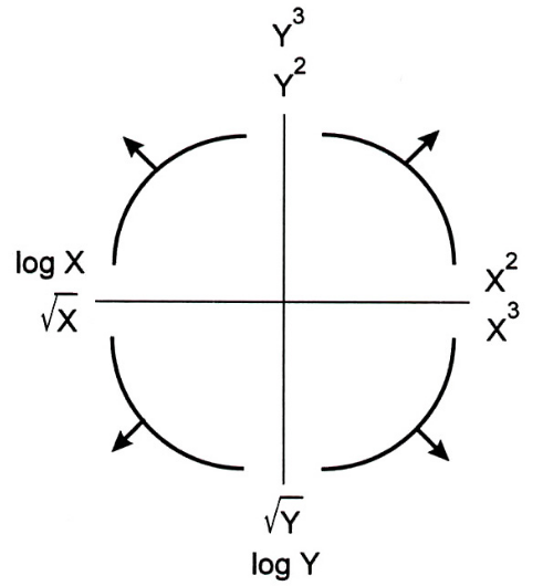
The bottom-left quadrant appears to match the shape of the scatter plot between 'horsepower' and 'mpg' the best – let's try taking the log of 'horsepower' ($X$).

mpg['log hp'] = np.log(mpg['horsepower'])

What does our data look like now?

px.scatter(mpg, x='log hp', y='mpg')

Predicting 'mpg' using log('horsepower')

Let's fit another linear model.

car_model_log = LinearRegression()
car_model_log.fit(mpg[['log hp']], mpg['mpg'])

LinearRegression()

What do our predictions look like now?

fig = px.scatter(mpg, x='log hp', y='mpg')
log_hp_points = pd.DataFrame({'log hp': [3.7, 5.5]})
fig = px.scatter(mpg, x='log hp', y='mpg')
fig.add_trace(go.Scatter(
    x=log_hp_points['log hp'],
    y=car_model_log.predict(log_hp_points),
    mode='lines',
    name='Predicted MPG using log(Horsepower)'
))

The fit looks a bit better! How about the $R^2$?

car_model_log.score(mpg[['log hp']], mpg['mpg'])

0.6683347641192137

Also a bit better!

What do our predictions look like on the original, non-transformed scatter plot? Let's see:

fig = px.scatter(mpg, x='horsepower', y='mpg')
fig.add_trace(
    go.Scatter(
        x=mpg['horsepower'], 
        y=car_model_log.intercept_ + car_model_log.coef_[0] * np.log(mpg['horsepower']),  
        mode='markers', name='Predicted MPG using log(Horsepower)', marker_color='red'
    )
)
fig

Our predictions that used $\log(\text{Horsepower})$ as an input don't fall on a straight line. We shouldn't expect them to; the red dots come from:

$$\text{Predicted MPG} = 108.698 - 18.582 \cdot \log(\text{Horsepower})$$

car_model_log.intercept_, car_model_log.coef_

(108.69970699574486, array([-18.58]))

Quantitative scaling

Until now, feature transformations we've discussed so far have involved converting categorical variables into quantitative variables. However, our log transformation was an example of transforming a quantitative variable into a new quantitative variable; this practice is called quantitative scaling.

• Standardization: $x_i \rightarrow \frac{x_i - \bar{x}}{\sigma_x}$.
• Linearization via a non-linear transformation: e.g. $\text{log}$ and $\text{sqrt}$. See Lab 8 for more.
• Discretization: Convert data into percentiles (or more generally, quantiles).

🙋🙋🏽‍♀️ Questions?

https://app.sli.do/event/2LZSnXWNpGPiuVnCZMa5J8

The modeling process

The modeling process

1. Create (engineer) features to best reflect the "meaning" behind data.

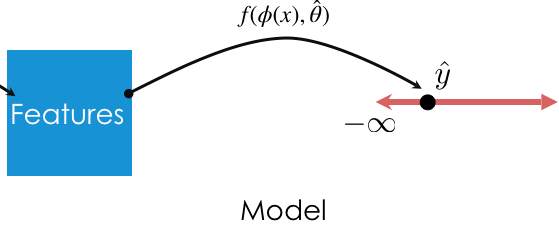
2. Choose a model that is appropriate to capture the relationships between features ($X$) and the target/response ($y$).

3. Select a loss function and fit the model (i.e., determine $w^*$).

4. Evaluate the model (e.g. using RMSE or $R^2$).

We can perform all of the above directly in sklearn!

preprocessing and linear_models

For the feature engineering step of the modeling pipeline, we will use sklearn's preprocessing module.

For the model creation step of the modeling pipeline, we will use sklearn's linear_model module, as we've already seen. linear_model.LinearRegression is an example of an estimator class.

Transformers in sklearn

Transformer classes

• Transformers take in "raw" data and output "processed" data. They are used for creating features.

• The input to a transformer should be a multi-dimensional numpy array.

  • Inputs can be DataFrames, but sklearn only looks at the values (i.e. it calls to_numpy() on input DataFrames).

• The output of a transformer is a numpy array (never a DataFrame or Series).

• Transformers, like most relevant features of sklearn, are classes, not functions, meaning you need to instantiate them and call their methods.

Case study: Restaurant tips 🧑‍🍳

We'll continue working with our trusty tips dataset.

tips.head()

	total_bill	tip	sex	smoker	...	time	size	smoker == Yes	smoker == No
0	3.07	1.00	Female	Yes	...	Dinner	1	1	0
1	18.78	3.00	Female	No	...	Dinner	2	0	1
2	26.59	3.41	Male	Yes	...	Dinner	3	1	0
3	14.26	2.50	Male	No	...	Lunch	2	0	1
4	21.16	3.00	Male	No	...	Lunch	2	0	1

5 rows × 9 columns

Example transformer: Binarizer

The Binarizer transformer allows us to map a quantitative sequence to a sequence of 1s and 0s, depending on whether values are above or below a threshold.

Property	Example	Description
Initialize with parameters	binar = Binarizer(thresh)	set x=1 if x > thresh, else 0
Transform data in a dataset	feat = binar.transform(data)	Binarize all columns in data

First, we need to import the relevant class from sklearn.preprocessing. (Tip: import just the relevant classes you need from sklearn.)

from sklearn.preprocessing import Binarizer

Let's try binarizing 'total_bill'. We'll say a "large" bill is one that is strictly greater than $20.

tips['total_bill'].head()

0     3.07
1    18.78
2    26.59
3    14.26
4    21.16
Name: total_bill, dtype: float64

First, we initialize a Binarizer object with the threshold we want.

bi = Binarizer(threshold=20)

Then, we call bi's transform method and pass it the data we'd like to transform. Note that its input and output are both 2D.

transformed_bills = bi.transform(tips[['total_bill']]) # Must give transform a 2D array/DataFrame.
transformed_bills[:5]

/Users/sam/mambaforge/envs/dsc80/lib/python3.8/site-packages/sklearn/base.py:443: UserWarning:

X has feature names, but Binarizer was fitted without feature names

array([[0.],
       [0.],
       [1.],
       [0.],
       [1.]])

Example transformer: StdScaler

• StdScaler standardizes data using the mean and standard deviation of the data.

$$z(x_i) = \frac{x_i - \text{mean of } x}{\text{SD of } x}$$

• Unlike Binarizer, StdScaler requires some knowledge (mean and SD) of the dataset before transforming.

• As such, we need to fit an StdScaler transformer before we can use the transform method.

• Typical usage: fit transformer on a sample, use that fit transformer to transform future data.

Example transformer: StdScaler

It only makes sense to standardize the already-quantitative features of tips, so let's select just those.

tips_quant = tips[['total_bill', 'size']]
tips_quant.head()

	total_bill	size
0	3.07	1
1	18.78	2
2	26.59	3
3	14.26	2
4	21.16	2

Let's initialize a StandardScaler object.

from sklearn.preprocessing import StandardScaler

stdscaler = StandardScaler()

Note that the following does not work! The error message is very helpful.

stdscaler.transform(tips_quant)

---------------------------------------------------------------------------
NotFittedError                            Traceback (most recent call last)
Cell In[48], line 1
----> 1 stdscaler.transform(tips_quant)

File ~/mambaforge/envs/dsc80/lib/python3.8/site-packages/sklearn/preprocessing/_data.py:970, in StandardScaler.transform(self, X, copy)
    955 def transform(self, X, copy=None):
    956     """Perform standardization by centering and scaling.
    957 
    958     Parameters
   (...)
    968         Transformed array.
    969     """
--> 970     check_is_fitted(self)
    972     copy = copy if copy is not None else self.copy
    973     X = self._validate_data(
    974         X,
    975         reset=False,
   (...)
    980         force_all_finite="allow-nan",
    981     )

File ~/mambaforge/envs/dsc80/lib/python3.8/site-packages/sklearn/utils/validation.py:1222, in check_is_fitted(estimator, attributes, msg, all_or_any)
   1217     fitted = [
   1218         v for v in vars(estimator) if v.endswith("_") and not v.startswith("__")
   1219     ]
   1221 if not fitted:
-> 1222     raise NotFittedError(msg % {"name": type(estimator).__name__})

NotFittedError: This StandardScaler instance is not fitted yet. Call 'fit' with appropriate arguments before using this estimator.

Instead, we need to first call the fit method on stdscaler.

# This is like saying "determine the mean and SD of each column in tips_quant".
stdscaler.fit(tips_quant)

StandardScaler()

Now, transform will work.

# First column is 'total_bill', second column is 'size'.
tips_quant_z = stdscaler.transform(tips_quant)
tips_quant_z[:5]

array([[-1.88, -1.65],
       [-0.11, -0.6 ],
       [ 0.77,  0.45],
       [-0.62, -0.6 ],
       [ 0.15, -0.6 ]])

We can also access the mean and variance stdscaler computed for each column:

stdscaler.mean_

array([19.79,  2.57])

stdscaler.var_

array([78.93,  0.9 ])

Note that we can call transform on DataFrames other than tips_quant. We will do this often – fit a transformer on one dataset (training data) and use it to transform other datasets (test data).

stdscaler.transform(tips_quant.sample(5))

array([[ 0.97, -0.6 ],
       [-0.28, -0.6 ],
       [ 1.19,  1.51],
       [-0.49, -0.6 ],
       [ 0.65,  1.51]])

💡 Pro-Tip: Using .fit_transform

The .fit_transform method will fit the transformer and then transform the data in one go.

stdscaler.fit_transform(tips_quant)

array([[-1.88, -1.65],
       [-0.11, -0.6 ],
       [ 0.77,  0.45],
       ...,
       [-0.26, -0.6 ],
       [-1.09, -0.6 ],
       [-0.32,  0.45]])

StdScaler summary

Property	Example	Description
Initialize with parameters	stdscaler = StandardScaler()	z-score the data (no parameters)
Fit the transformer	stdscaler.fit(X)	Compute the mean and SD of X
Transform data in a dataset	feat = stdscaler.transform(X_new)	z-score X_new with mean and SD of X
Fit and transform	stdscaler.fit_transform(X)	Compute the mean and SD of X, then z-score X

Example transformer: OneHotEncoder

Let's keep just the categorical columns in tips.

tips_cat = tips[['sex', 'smoker', 'day', 'time']]
tips_cat.head()

	sex	smoker	day	time
0	Female	Yes	Sat	Dinner
1	Female	No	Thur	Dinner
2	Male	Yes	Sat	Dinner
3	Male	No	Thur	Lunch
4	Male	No	Thur	Lunch

Like StdScaler, we will need to fit our OneHotEncoder transformer before it can transform anything.

from sklearn.preprocessing import OneHotEncoder

ohe = OneHotEncoder()
ohe.fit(tips_cat)

OneHotEncoder()

We can look at the unique values (i.e. categories) in each column by using the categories_ attribute:

ohe.categories_

[array(['Female', 'Male'], dtype=object),
 array(['No', 'Yes'], dtype=object),
 array(['Fri', 'Sat', 'Sun', 'Thur'], dtype=object),
 array(['Dinner', 'Lunch'], dtype=object)]

ohe.transform(tips_cat)

<244x10 sparse matrix of type '<class 'numpy.float64'>'
	with 976 stored elements in Compressed Sparse Row format>

Since the resulting matrix is sparse – most of its elements are 0 – sklearn uses a more efficient representation than a regular numpy array. We can convert to a regular (dense) array:

ohe.transform(tips_cat).toarray()

array([[1., 0., 0., ..., 0., 1., 0.],
       [1., 0., 1., ..., 1., 1., 0.],
       [0., 1., 0., ..., 0., 1., 0.],
       ...,
       [1., 0., 1., ..., 1., 0., 1.],
       [0., 1., 1., ..., 0., 1., 0.],
       [1., 0., 1., ..., 0., 1., 0.]])

Notice that the column names from tips_cat are no longer stored anywhere (remember, fit converts the input to a numpy array before proceeding).

We can use the get_feature_names_out method on ohe to access the names of the one-hot-encoded columns, though:

ohe.get_feature_names_out() # x0, x1, x2, and x3 correspond to column names in tips_cat.

array(['sex_Female', 'sex_Male', 'smoker_No', 'smoker_Yes', 'day_Fri',
       'day_Sat', 'day_Sun', 'day_Thur', 'time_Dinner', 'time_Lunch'],
      dtype=object)

pd.DataFrame(ohe.transform(tips_cat).toarray(), 
             columns=ohe.get_feature_names_out()) # If we need a DataFrame back, for some reason.

	sex_Female	sex_Male	smoker_No	smoker_Yes	...	day_Sun	day_Thur	time_Dinner	time_Lunch
0	1.0	0.0	0.0	1.0	...	0.0	0.0	1.0	0.0
1	1.0	0.0	1.0	0.0	...	0.0	1.0	1.0	0.0
2	0.0	1.0	0.0	1.0	...	0.0	0.0	1.0	0.0
...	...	...	...	...	...	...	...	...	...
241	1.0	0.0	1.0	0.0	...	0.0	1.0	0.0	1.0
242	0.0	1.0	1.0	0.0	...	0.0	0.0	1.0	0.0
243	1.0	0.0	1.0	0.0	...	0.0	0.0	1.0	0.0

244 rows × 10 columns

Pipelines

So far, we've used transformers for feature engineering and models for prediction. We can combine these steps into a single Pipeline.

Pipelines in sklearn

• To instantiate a Pipeline, we must provide a list with zero or more transformers followed by a single model.

  • All "steps" must have fit methods, and all but the last must have transform methods.
  • Template: pl = Pipeline([feat_trans1, feat_trans2, ..., mdl]).

• Once a Pipeline is instantiated, you can fit all steps (transformers and model) using a single call to the fit method.

pl.fit(X, y)

• To make predictions using raw, untransformed data, use pl.predict.

• The actual list we provide Pipeline with must be a list of tuples, where

  • The first element is a "name" (that we choose) for the step.
  • The second element is a transformer or estimator instance.

Our first Pipeline

Let's build a Pipeline that:

• One hot encodes the categorical features in tips.
• Fits a regression model on the one hot encoded data.

tips_cat = tips[['sex', 'smoker', 'day', 'time']]
tips_cat.head()

	sex	smoker	day	time
0	Female	Yes	Sat	Dinner
1	Female	No	Thur	Dinner
2	Male	Yes	Sat	Dinner
3	Male	No	Thur	Lunch
4	Male	No	Thur	Lunch

from sklearn.pipeline import Pipeline

pl = Pipeline([
    ('one-hot', OneHotEncoder()),
    ('lin-reg', LinearRegression())
])

Now that pl is instantiated, we fit it the same way we would fit the individual steps.

pl.fit(tips_cat, tips['tip'])

Pipeline(steps=[('one-hot', OneHotEncoder()), ('lin-reg', LinearRegression())])

Now, to make predictions using raw data, all we need to do is use pl.predict:

pl.predict(tips_cat.iloc[:5])

array([2.92, 3.16, 3.09, 2.83, 2.83])

pl performs both feature transformation and prediction with just a single call to predict!

We can access individual "steps" of a Pipeline through the named_steps attribute:

pl.named_steps

{'one-hot': OneHotEncoder(), 'lin-reg': LinearRegression()}

pl.named_steps['one-hot'].transform(tips_cat).toarray()

array([[1., 0., 0., ..., 0., 1., 0.],
       [1., 0., 1., ..., 1., 1., 0.],
       [0., 1., 0., ..., 0., 1., 0.],
       ...,
       [1., 0., 1., ..., 1., 0., 1.],
       [0., 1., 1., ..., 0., 1., 0.],
       [1., 0., 1., ..., 0., 1., 0.]])

pl.named_steps['lin-reg'].coef_

array([-0.09,  0.09, -0.04,  0.04, -0.2 , -0.13,  0.14,  0.19,  0.25,
       -0.25])

pl also has a score method, the same way a fit LinearRegression instance does:

pl.score(tips_cat, tips['tip'])

0.02749679020147533

More sophisticated Pipelines

• In the previous example, we one hot encoded every input column. What if we want to perform different transformations on different columns?

• Solution: Use a ColumnTransformer.

  • Instantiate a ColumnTransformer using a list of tuples, where:
    • The first element is a "name" we choose for the transformer.
    • The second element is a transformer instance (e.g. OneHotEncoder()).
    • The third element is a list of relevant column names.

Planning our first ColumnTransformer

from sklearn.compose import ColumnTransformer

Let's perform different transformations on the quantitative and categorical features of tips (note that we are not transforming 'tip').

tips_features = tips.drop('tip', axis=1)
tips_features.head()

	total_bill	sex	smoker	day	time	size	smoker == Yes	smoker == No
0	3.07	Female	Yes	Sat	Dinner	1	1	0
1	18.78	Female	No	Thur	Dinner	2	0	1
2	26.59	Male	Yes	Sat	Dinner	3	1	0
3	14.26	Male	No	Thur	Lunch	2	0	1
4	21.16	Male	No	Thur	Lunch	2	0	1

• We will leave the 'total_bill' column untouched.

• To the 'size' column, we will apply the Binarizer transformer with a threshold of 2 (big tables vs. small tables).

• To the categorical columns, we will apply the OneHotEncoder transformer.

• In essence, we will create a transformer that reproduces the following DataFrame:

	size	x0_Female	x0_Male	x1_No	x1_Yes	x2_Fri	x2_Sat	x2_Sun	x2_Thur	x3_Dinner	x3_Lunch	total_bill
0	0	1.0	0.0	1.0	0.0	0.0	0.0	1.0	0.0	1.0	0.0	16.99
1	1	0.0	1.0	1.0	0.0	0.0	0.0	1.0	0.0	1.0	0.0	10.34
2	1	0.0	1.0	1.0	0.0	0.0	0.0	1.0	0.0	1.0	0.0	21.01
3	0	0.0	1.0	1.0	0.0	0.0	0.0	1.0	0.0	1.0	0.0	23.68
4	1	1.0	0.0	1.0	0.0	0.0	0.0	1.0	0.0	1.0	0.0	24.59

Building a Pipeline using a ColumnTransformer

Let's start by creating our ColumnTransformer.

preproc = ColumnTransformer(
    transformers=[
        ('size', Binarizer(threshold=2), ['size']),
        ('categorical_cols', OneHotEncoder(), ['sex', 'smoker', 'day', 'time'])
    ],
    remainder='passthrough' # Specify what to do with all other columns ('total_bill' here) – drop or passthrough.
)

Now, let's create a Pipeline using preproc as a transformer, and fit it:

pl = Pipeline([
    ('preprocessor', preproc), 
    ('lin-reg', LinearRegression())
])

pl.fit(tips_features, tips['tip'])

Pipeline(steps=[('preprocessor',
                 ColumnTransformer(remainder='passthrough',
                                   transformers=[('size',
                                                  Binarizer(threshold=2),
                                                  ['size']),
                                                 ('categorical_cols',
                                                  OneHotEncoder(),
                                                  ['sex', 'smoker', 'day',
                                                   'time'])])),
                ('lin-reg', LinearRegression())])

Prediction is as easy as calling predict:

tips_features.head()

	total_bill	sex	smoker	day	time	size	smoker == Yes	smoker == No
0	3.07	Female	Yes	Sat	Dinner	1	1	0
1	18.78	Female	No	Thur	Dinner	2	0	1
2	26.59	Male	Yes	Sat	Dinner	3	1	0
3	14.26	Male	No	Thur	Lunch	2	0	1
4	21.16	Male	No	Thur	Lunch	2	0	1

# Note that we fit the Pipeline using tips_features, not tips_features.head()!
pl.predict(tips_features.head())

array([1.16, 2.81, 3.7 , 2.4 , 3.07])

Aside: FunctionTransformer

A transformer you'll often use as part of a ColumnTransformer is the FunctionTransformer, which enables you to use your own functions on entire columns. Think of it as the sklearn equivalent of apply.

from sklearn.preprocessing import FunctionTransformer

f = FunctionTransformer(np.sqrt)
f.transform([1, 2, 3])

array([1.  , 1.41, 1.73])

Summary: Pipelines

• Pipelines are powerful because they allow you to perform feature engineering and training/prediction all through a single object.
• As we'll see next time, they also allow us to easily compare models against each other.

🙋🙋🏽‍♀️ Questions?

https://app.sli.do/event/2LZSnXWNpGPiuVnCZMa5J8

Generalization

Motivation

• You and Billy are studying for an upcoming exam. You both decide to test your understanding by taking a practice exam.

  • Your logic: If you do well on the practice exam, you should do well on the real exam.

• You each take the practice exam once and look at the solutions afterwards.

• Your strategy: Memorize the answers to all practice exam questions, e.g. "Question 1: A; Question 2: C; Question 3: A."

• Billy's strategy: Learn high-level concepts from the solutions, e.g. "data are NMAR if the likelihood of missingness depends on the missing values themselves."

• Who will do better on the practice exam? Who will probably do better on the real exam? 🧐

Evaluating the quality of a model

• So far, we've computed the RMSE (and $R^2$) of our fit regression models on the data that we used to fit them, i.e. the training data.

• We've said that Model A is better than Model B if Model A's RMSE is lower than Model B's RMSE.

  • Remember, our training data is a sample from the data generating process.
  • Just because a model fits the training data well doesn't mean it will generalize and work well on similar, unseen samples!

Example: Overfitting and underfitting

Let's collect two samples $\{(x_i, y_i)\}$ from the same data generating process.

np.random.seed(23) # For reproducibility.

def sample_dgp(n=100):
    x = np.linspace(-2, 3, n)
    y = x ** 3 + (np.random.normal(0, 3, size=n))
    return pd.DataFrame({'x': x, 'y': y})

sample_1 = sample_dgp()
sample_2 = sample_dgp()

For now, let's just look at Sample 1. The relationship between $x$ and $y$ is roughly cubic; that is, $y \approx x^3$ (remember, in reality, you won't get to see the DGP).

px.scatter(sample_1, x='x', y='y', title='Sample 1')

Polynomial regression

Let's fit three polynomial models on Sample 1:

• Degree 1.
• Degree 3.
• Degree 25.

The PolynomialFeatures transformer will be helpful here.

from sklearn.preprocessing import PolynomialFeatures

# fit_transform fits and transforms the same input.
d2 = PolynomialFeatures(3)
d2.fit_transform(np.array([1, 2, 3, 4, -2]).reshape(-1, 1))

array([[ 1.,  1.,  1.,  1.],
       [ 1.,  2.,  4.,  8.],
       [ 1.,  3.,  9., 27.],
       [ 1.,  4., 16., 64.],
       [ 1., -2.,  4., -8.]])

Below, we look at our three models' predictions on Sample 1 (which they were trained on).

# Look at the definition of train_and_plot in util.py if you're curious as to how the plotting works.
import lec14_util as util
fig = util.train_and_plot(train_sample=sample_1, test_sample=sample_1, degs=[1, 3, 25])
fig.update_layout(title='Trained on Sample 1, Performance on Sample 1')

The degree 25 polynomial has the lowest RMSE on Sample 1.

How do the same fit polynomials look on Sample 2?

fig = util.train_and_plot(train_sample=sample_1, test_sample=sample_2, degs=[1, 3, 25])
fig.update_layout(title='Trained on Sample 1, Performance on Sample 2')

• The degree 3 polynomial has the lowest RMSE on Sample 2.

• Note that we didn't get to see Sample 2 when fitting our models!

• As such, it seems that the degree 3 polynomial generalizes better to unseen data than the degree 25 polynomial does.

What if we fit a degree 1, degree 3, and degree 25 polynomial on Sample 2 as well?

util.plot_multiple_models(sample_1, sample_2, degs=[1, 3, 25])

Key idea: Degree 25 polynomials seem to vary more when trained on different samples than degree 3 and 1 polynomials do.

• Next time: We'll investigate this phenomenon in-depth, and introduce techniques for choosing the best model.