from dsc80_utils import *
# Carryover setup from last lecture
import seaborn as sns
tips = sns.load_dataset('tips')

from sklearn.linear_model import LinearRegression

import lec15_util as util
📣 Announcements 📣
- Project 4 out, due this Friday, Dec 1.
- Start early! Historically, the last two questions of the project take up about 75% of the project time.
- Lab 9 out, due Dec 4. (The last lab!)
📆 Agenda
- Multicollinearity
- Why we drop one column when using one-hot encoding
- Generalization
- Cross-validation

Multicollinearity
people = pd.read_csv('data/SOCR-HeightWeight.csv').drop(columns=['Index'])
people.head()
| Height (Inches) | Weight (Pounds) | |
|---|---|---|
| 0 | 65.78 | 112.99 |
| 1 | 71.52 | 136.49 |
| 2 | 69.40 | 153.03 |
| 3 | 68.22 | 142.34 |
| 4 | 67.79 | 144.30 |
people.plot(kind='scatter', x='Height (Inches)', y='Weight (Pounds)',
            title='Weight vs. Height for 25,000 18 Year Olds')
Motivating example
Suppose we fit a simple linear regression model that uses height in inches to predict weight in pounds.
$$\text{predicted weight (pounds)} = w_0 + w_1 \cdot \text{height (inches)}$$from sklearn.linear_model import LinearRegression
from sklearn.metrics import mean_squared_error
X = people[['Height (Inches)']]
y = people['Weight (Pounds)']
lr_one_feat = LinearRegression()
lr_one_feat.fit(X, y)
LinearRegression()
$w_0^*$ and $w_1^*$ are shown below, along with the model's training set RMSE.
lr_one_feat.intercept_, lr_one_feat.coef_
(-82.57574306454099, array([3.08]))
rmse_one_feat = mean_squared_error(
    y, lr_one_feat.predict(X), squared=False
)
rmse_one_feat
10.079113675632819
Now, suppose we fit another regression model, that uses height in inches AND height in centimeters to predict weight.
$$\text{predicted weight (pounds)} = w_0 + w_1 \cdot \text{height (inches)} + w_2 \cdot \text{height (cm)}$$people['Height (cm)'] = people['Height (Inches)'] * 2.54 # 1 inch = 2.54 cm
X2 = people[['Height (Inches)', 'Height (cm)']]
lr_two_feat = LinearRegression()
lr_two_feat.fit(X2, y)
LinearRegression()
What are $w_0^*$, $w_1^*$, $w_2^*$, and the model's testing RMSE?
lr_two_feat.intercept_, lr_two_feat.coef_
(-82.57585227669999, array([-2.46e+10, 9.67e+09]))
rmse_two_feat = mean_squared_error(
    y, lr_two_feat.predict(X2), squared=False)
rmse_two_feat
10.079113005376787
Observation: The intercept is the same as before (roughly -81.17), as is the testing RMSE. However, the coefficients on 'Height (Inches)' and 'Height (cm)' are massive in size!
What's going on?
Redundant features
Let's use simpler numbers for illustration. Suppose in the first model, $w_0^* = -80$ and $w_1^* = 3$.
In the second model, we have:
$$\begin{align*}\text{predicted weight (pounds)} &= w_0^* + w_1^* \cdot \text{height (inches)} + w_2^* \cdot \text{height (cm)} \\ &= w_0^* + w_1^* \cdot \text{height (inches)} + w_2^* \cdot \big( 2.54^* \cdot \text{height (inches)} \big) \\ &= w_0^* + \left(w_1^* + 2.54 \cdot w_2^* \right) \cdot \text{height (inches)} \end{align*}$$In the first model, we already found the "best" intercept ($-80$) and slope ($3$) in a linear model that uses height in inches to predict weight.
So, as long as $w_1^* + 2.54 \cdot w_2^* = 3$ in the second model, the second model's training predictions will be the same as the first, and hence they will also minimize RMSE.
Infinitely many parameter choices
Issue: There are an infinite number of $w_1^*$ and $w_2^*$ that satisfy $w_1^* + 2.54 \cdot w_2^* = 3$!
- Both prediction rules look very different, but actually make the same predictions.
lr.coef_could return either set of coefficients, or any other of the infinitely many options.
- But neither set of coefficients is has any meaning!
(-80 - 10 * people.iloc[:, 0] + (13 / 2.54) * people.iloc[:, 2]).head()
0    117.35
1    134.55
2    128.20
3    124.65
4    123.36
dtype: float64
(-80 + 10 * people.iloc[:, 0] - (7 / 2.54) * people.iloc[:, 2]).head()
0    117.35
1    134.55
2    128.20
3    124.65
4    123.36
dtype: float64
Multicollinearity
Multicollinearity occurs when features in a regression model are highly correlated with one another.
- In other words, multicollinearity occurs when a feature can be predicted using a linear combination of other features, fairly accurately.
When multicollinearity is present in the features, the coefficients in the model are uninterpretable – they have no meaning.
- A "slope" represents "the rate of change of $y$ with respect to a feature", when all other features are held constant – but if there's multicollinearity, you can't hold other features constant.
Note: Multicollinearity doesn't impact a model's predictions!
- It doesn't impact a model's ability to generalize to unseen data.
- If features are multicollinear in the training data, they will probably be multicollinear in the test data too.
Solutions:
- Manually remove highly correlated features.
- Use a dimensionality reduction technique (such as PCA) to automatically reduce dimensions.
Key takeaways
- Multicollinearity is present in a linear model when one feature can be accurately predicted using one or more other features.
- In other words, it is present when a feature is redundant.
- Multicollinearity doesn't pose an issue for prediction; it doesn't hinder a model's ability to generalize. Instead, it renders the coefficients of a linear model meaningless.
Example: One-hot encoding
A one-hot encoding will result in multicollinearity unless you drop one of the one-hot encoded features.
Suppose we have the following fitted model:
$$ \begin{aligned} H(x) = 1 + 2 \cdot (\text{smoker==Yes}) - 2 \cdot (\text{smoker==No}) \end{aligned} $$This is equivalent to:
$$ \begin{aligned} H(x) = 10 - 7 \cdot (\text{smoker==Yes}) - 11 \cdot (\text{smoker==No}) \end{aligned} $$Solution: Drop one of the one-hot encoded columns. sklearn.preprocessing.OneHotEncoder has an option to do this.
Generalization
Example: Overfitting and underfitting
Let's collect two samples $\{(x_i, y_i)\}$ from the same data generating process.
np.random.seed(23) # For reproducibility.

def sample_dgp(n=100):
    x = np.linspace(-2, 3, n)
    y = x ** 3 + (np.random.normal(0, 3, size=n))
    return pd.DataFrame({'x': x, 'y': y})

sample_1 = sample_dgp()
sample_2 = sample_dgp()
For now, let's just look at Sample 1. The relationship between $x$ and $y$ is roughly cubic; that is, $y \approx x^3$ (remember, in reality, you won't get to see the DGP).
px.scatter(sample_1, x='x', y='y', title='Sample 1')
Polynomial regression
Let's fit three polynomial models on Sample 1:
- Degree 1.
- Degree 3.
- Degree 25.
The PolynomialFeatures transformer will be helpful here.
from sklearn.preprocessing import PolynomialFeatures
# fit_transform fits and transforms the same input.
d2 = PolynomialFeatures(3)
d2.fit_transform(np.array([1, 2, 3, 4, -2]).reshape(-1, 1))
array([[ 1.,  1.,  1.,  1.],
       [ 1.,  2.,  4.,  8.],
       [ 1.,  3.,  9., 27.],
       [ 1.,  4., 16., 64.],
       [ 1., -2.,  4., -8.]])
Below, we look at our three models' predictions on Sample 1 (which they were trained on).
# Look at the definition of train_and_plot in lec15_util.py if you're curious as to how the plotting works.
fig = util.train_and_plot(train_sample=sample_1, test_sample=sample_1, degs=[1, 3, 25])
fig.update_layout(title='Trained on Sample 1, Performance on Sample 1')
The degree 25 polynomial has the lowest RMSE on Sample 1.
How do the same fit polynomials look on Sample 2?
fig = util.train_and_plot(train_sample=sample_1, test_sample=sample_2, degs=[1, 3, 25])
fig.update_layout(title='Trained on Sample 1, Performance on Sample 2')
The degree 3 polynomial has the lowest RMSE on Sample 2.
Note that we didn't get to see Sample 2 when fitting our models!
As such, it seems that the degree 3 polynomial generalizes better to unseen data than the degree 25 polynomial does.
What if we fit a degree 1, degree 3, and degree 25 polynomial on Sample 2 as well?
util.plot_multiple_models(sample_1, sample_2, degs=[1, 3, 25])
Key idea: Degree 25 polynomials seem to vary more when trained on different samples than degree 3 and 1 polynomials do.
Bias and variance
The training data we have access to is a sample from the DGP. We are concerned with our model's ability to generalize and work well on different datasets drawn from the same DGP.
Suppose we fit a model $H$ (e.g. a degree 3 polynomial) on several different datasets from a DGP. There are three sources of error that arise:
- ⭐️ Bias: The expected deviation between a predicted value and an actual value.
- In other words, for a given $x_i$, how far is $H(x_i)$ from the true $y_i$, on average?
- Low bias is good! ✅
- High bias is a sign of underfitting, i.e. that our model is too basic to capture the relationship between our features and response.
⭐️ Model variance ("variance"): The variance of a model's predictions.
- In other words, for a given $x_i$, what is the variance of $H(x_i)$ across all datasets?
- Low model variance is good! ✅
- High model variance is a sign of overfitting, i.e. that our model is too complicated and is prone to fitting to the noise in our training data.
Observation variance: The variance due to the random noise in the process we are trying to model (e.g. measurement error). We can't control this, without collecting more data!
Here, suppose:
- The red bulls-eye represents your true weight and height 🧍.
- The dark blue darts represent predictions of your weight and height using different models that were fit on the same DGP.
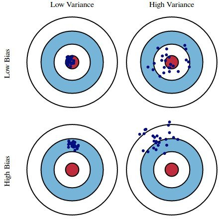
We'd like our models to be in the top left, but in practice that's hard to achieve!
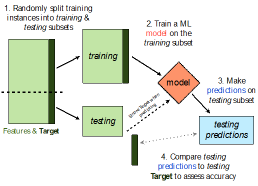
Train-test split
Avoiding overfitting
We won't know whether our model has overfit to our sample (training data) unless we get to see how well it performs on a new sample from the same DGP.
💡Idea: Split our sample into a training set and test set.
Use only the training set to fit the model (i.e. find $w^*$).
Use the test set to evaluate the model's error (RMSE, $R^2$).
The test set is like a new sample of data from the same DGP as the training data!
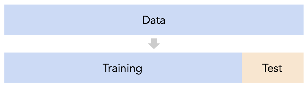
Train-test split 🚆
sklearn.model_selection.train_test_split implements a train-test split for us! 🙏🏼
If X is an array/DataFrame of features and y is an array/Series of responses,
X_train, X_test, y_train, y_test = train_test_split(X, y, test_size=0.25)
randomly splits the features and responses into training and test sets, such that the test set contains 0.25 of the full dataset.
from sklearn.model_selection import train_test_split
# Read the documentation!
train_test_split?
Let's perform a train/test split on our tips dataset.
X = tips.drop('tip', axis=1)
y = tips['tip']
X_train, X_test, y_train, y_test = train_test_split(X, y, test_size=0.2) # We don't have to choose 0.25.
Before proceeding, let's check the sizes of X_train and X_test.
print('Rows in X_train:', X_train.shape[0])
display(X_train.head())
print('Rows in X_test:', X_test.shape[0])
display(X_test.head())
Rows in X_train: 195
| total_bill | sex | smoker | day | time | size | |
|---|---|---|---|---|---|---|
| 4 | 24.59 | Female | No | Sun | Dinner | 4 |
| 209 | 12.76 | Female | Yes | Sat | Dinner | 2 |
| 178 | 9.60 | Female | Yes | Sun | Dinner | 2 |
| 230 | 24.01 | Male | Yes | Sat | Dinner | 4 |
| 5 | 25.29 | Male | No | Sun | Dinner | 4 |
Rows in X_test: 49
| total_bill | sex | smoker | day | time | size | |
|---|---|---|---|---|---|---|
| 146 | 18.64 | Female | No | Thur | Lunch | 3 |
| 224 | 13.42 | Male | Yes | Fri | Lunch | 2 |
| 134 | 18.26 | Female | No | Thur | Lunch | 2 |
| 131 | 20.27 | Female | No | Thur | Lunch | 2 |
| 147 | 11.87 | Female | No | Thur | Lunch | 2 |
X_train.shape[0] / tips.shape[0]
0.7991803278688525
Example train-test split
Steps:
- Fit a model on the training set.
- Evaluate the model on the test set.
tips.head()
| total_bill | tip | sex | smoker | day | time | size | |
|---|---|---|---|---|---|---|---|
| 0 | 16.99 | 1.01 | Female | No | Sun | Dinner | 2 |
| 1 | 10.34 | 1.66 | Male | No | Sun | Dinner | 3 |
| 2 | 21.01 | 3.50 | Male | No | Sun | Dinner | 3 |
| 3 | 23.68 | 3.31 | Male | No | Sun | Dinner | 2 |
| 4 | 24.59 | 3.61 | Female | No | Sun | Dinner | 4 |
X = tips[['total_bill', 'size']] # For this example, we'll use just the already-quantitative columns in tips.
y = tips['tip']
X_train, X_test, y_train, y_test = train_test_split(X, y, test_size=0.2, random_state=1) # random_state is like np.random.seed.
Here, we'll use a stand-alone LinearRegression model without a Pipeline, but this process would work the same if we were using a Pipeline.
lr = LinearRegression()
lr.fit(X_train, y_train)
LinearRegression()
Let's check our model's performance on the training set first.
from sklearn.metrics import mean_squared_error # Built-in RMSE/MSE function.
pred_train = lr.predict(X_train)
rmse_train = mean_squared_error(y_train, pred_train, squared=False)
rmse_train
0.9803205287924737
And the test set:
pred_test = lr.predict(X_test)
rmse_test = mean_squared_error(y_test, pred_test, squared=False)
rmse_test
1.138177129113125
Since rmse_train and rmse_test are similar, it doesn't seem like our model is overfitting to the training data. If rmse_test was much larger than rmse_train, it would be evidence that our model is unable to generalize well.
Hyperparameters
Example: Polynomial regression
We recently looked at an example of polynomial regression.
fig = util.train_and_plot(train_sample=sample_1, test_sample=sample_2, degs=[1, 3, 25])
fig.update_layout(title='Trained on Sample 1, Performance on Sample 2')
When building these models:
- We got to choose the degree of the polynomials (i.e. we chose 1, 3, and 25).
- We didn't get to choose the exact formulas for the three polynomials – their formulas were learned from data.
Parameters vs. hyperparameters
A parameter defines the relationship between variables in a model.
- We learn parameters from data.
- For instance, suppose we fit a degree 3 polynomial to data, and end up with
$$H(x) = 1 - 2x + 13x^2 - 4x^3$$
- 1, -2, 13, and -4 are parameters.
A hyperparameter is a parameter that we get to choose before our model is fit to the data.
- Think of hyperparameters as knobs 🎛 – we get to pick and tune them!
- Polynomial degree was a hyperparameter in the previous example, and we tried three different values – 1, 3, and 25.
Question: How do we choose the "right" hyperparameter(s)?
Training error vs. test error
We know that a model's performance on a test set is a good estimate of its ability to generalize to unseen data.
We want to find the hyperparameter that leads to the best test set performance.
Idea:
- Come up with a list of hyperparameters to try.
- For each hyperparameter, train the model on the training set and compute its performance on the test set.
- Pick the hyperparameter with the best performance on the test set.
Training error vs. test error
Let's try this strategy on sample 1 from our earlier example.
We'll try to fit a polynomial model on the dataset; we'll choose the polynomial's degree from the list [1, 2, ..., 25].
px.scatter(sample_1, x='x', y='y', title='Sample 1')
First, we perform a train-test split.
X = sample_1[['x']]
y = sample_1['y']

X_train, X_test, y_train, y_test = train_test_split(X, y, random_state=100)
💡 Pro-Tip: Using make_pipeline
Instead of using the Pipeline class directly, you can use make_pipeline for a more compact syntax:
(Also, I like using the analogous sklearn.compose.make_column_transformer instead of the ColumnTransformer class.)
from sklearn.pipeline import Pipeline, make_pipeline
from sklearn.preprocessing import PolynomialFeatures
# Pipeline with degree-2 polynomial features
pl = Pipeline([('poly', PolynomialFeatures(2)), ('lin-reg', LinearRegression())])

# Same pipeline, notice that make_pipeline generates names for pipeline steps
pl = make_pipeline(PolynomialFeatures(2), LinearRegression())
pl
Pipeline(steps=[('polynomialfeatures', PolynomialFeatures()),
                ('linearregression', LinearRegression())])
Polynomial degree vs. train/test error
Now, we'll create models with degree-1 through degree-25 polynomial features and compute their train and test errors.
train_errs = []
test_errs = []

for d in range(1, 26):
    pl = make_pipeline(PolynomialFeatures(d), LinearRegression())
    pl.fit(X_train, y_train)
    train_errs.append(mean_squared_error(y_train, pl.predict(X_train), squared=False))
    test_errs.append(mean_squared_error(y_test, pl.predict(X_test), squared=False))

errs = pd.DataFrame({'Train Error': train_errs, 'Test Error': test_errs})
Let's look at the plots of training error vs. degree and test error vs. degree.
fig = px.line(errs)
fig.update_layout(showlegend=True, xaxis_title='Degree', yaxis_title='RMSE')
Training error appears to decrease as polynomial degree increases.
Test error appears to decrease until a "valley", and then increases again.
Here, we'd choose a degree of 3, since that degree has the lowest test error.
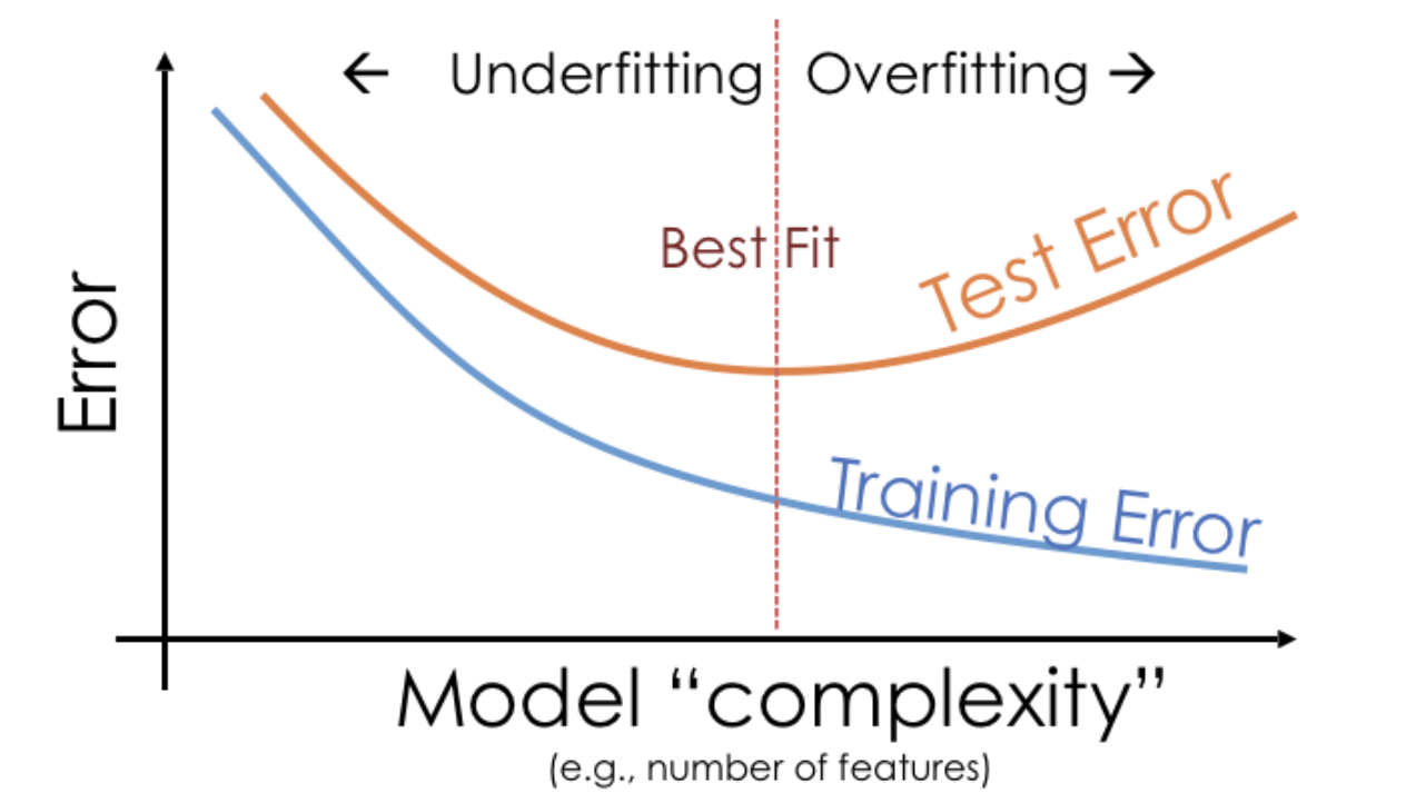
We pick the hyperparameter(s) at the "valley" of test error.
Note that training error tends to underestimate test error, but it doesn't have to – i.e., it is possible for test error to be lower than training error (say, if the test set is "easier" to predict than the training set).
Conducting train-test splits
- Recall, training data is used to fit our model, and test data is used to evaluate our model.
Question: How should we split?
sklearn'strain_test_splitsplits randomly, which usually works well.- However, if there is some element of time in the training data (say, when predicting the future price of a stock), a better split is "past" and "future".
Question: How large should the split be, e.g. 90%-10% vs. 75%-25%?
- There's a tradeoff – a larger training set should lead to a "better" model, while a larger test set should lead to a better estimate of our model's ability to generalize.
- There's no "right" choice, but we usually choose between 10% to 25% for the test set.
But wait...
With our current strategy, we are choosing the hyperparameter that creates the model that performs best on the test set.
As such, we are overfitting to the test set – the best hyperparameter for the test set might not be the best hyperparameter for a totally unseen dataset!
It seems like we need another split.
Cross-validation
A single validation set
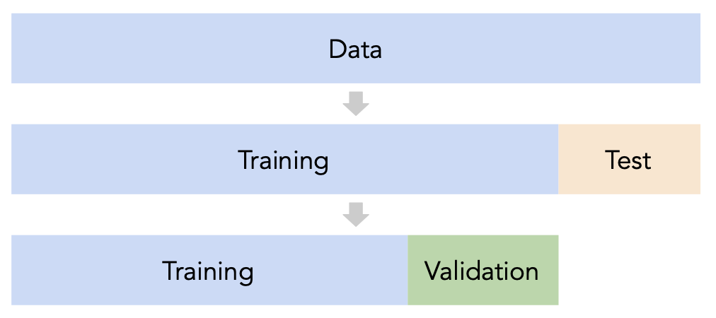
Split the data into three sets: training, validation, and test.
For each hyperparameter choice, train the model only on the training set, and evaluate the model's performance on the validation set.
Find the hyperparameter with the best validation performance.
Retrain the final model on the training and validation sets, and report its performance on the test set.
Issue: This strategy is too dependent on the validation set, which may be small and/or not a representative sample of the data.
$k$-fold cross-validation
Instead of relying on a single validation set, we can create $k$ validation sets, where $k$ is some positive integer (5 in the example below).
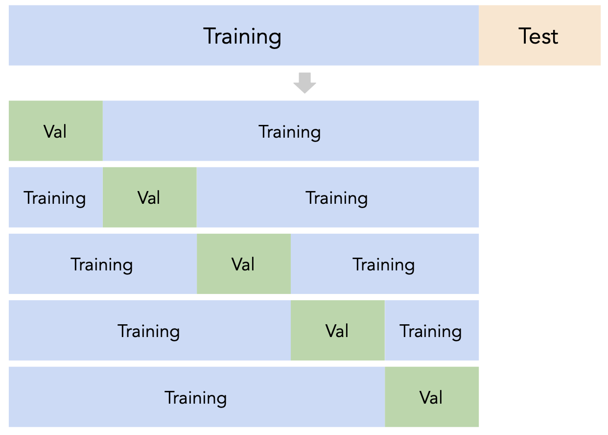
Since each data point is used for training $k-1$ times and validation once, the (averaged) validation performance should be a good metric of a model's ability to generalize to unseen data.
$k$-fold cross-validation (or simply "cross-validation") is the technique we will use for finding hyperparameters.
Creating folds in sklearn
sklearn has a KFold class that splits data into training and validation folds.
from sklearn.model_selection import KFold
Let's use a simple dataset for illustration.
data = np.arange(10, 70, 10)
data
array([10, 20, 30, 40, 50, 60])
Let's instantiate a KFold object with $k=3$.
kfold = KFold(3, shuffle=True, random_state=1)
kfold
KFold(n_splits=3, random_state=1, shuffle=True)
Finally, let's use kfold to split data:
for train, val in kfold.split(data):
    print(f'train: {data[train]}, validation: {data[val]}')
train: [10 40 50 60], validation: [20 30]
train: [20 30 40 60], validation: [10 50]
train: [10 20 30 50], validation: [40 60]
Note that each value in data is used for validation exactly once and for training exactly twice. Also note that because we set shuffle=True the groups are not simply [10, 20], [30, 40], and [50, 60].
$k$-fold cross-validation
First, shuffle the dataset randomly and split it into $k$ disjoint groups. Then:
- For each hyperparameter:
- For each unique group:
- Let the unique group be the "validation set".
- Let all other groups be the "training set".
- Train a model using the selected hyperparameter on the training set.
- Evaluate the model on the validation set.
- Compute the average validation score (e.g. RMSE) for the particular hyperparameter.
- For each unique group:
- Choose the hyperparameter with the best average validation score.
$k$-fold cross-validation in sklearn
While you could manually use KFold to perform cross-validation, the cross_val_score function in sklearn implements $k$-fold cross-validation for us!
cross_val_score(estimator, X_train, y_train, cv)
Specifically, it takes in:
- A
Pipelineor estimator that has not already beenfit. - Training data.
- A value of $k$ (through the
cvargument). - (Optionally) A
scoringmetric.
and performs $k$-fold cross-validation, returning the values of the scoring metric on each fold.
from sklearn.model_selection import cross_val_score
$k$-fold cross-validation in sklearn
Let's perform $k$-fold cross validation in order to help us pick a degree for polynomial regression from the list [1, 2, ..., 25].
We'll use $k=5$ since it's a common choice (and the default in
sklearn).For the sake of this example, we'll suppose
sample_1is our "training + validation data", i.e. that our test data is in some other dataset.- If this were not true, we'd first need to split
sample_1into separate training and test sets.
- If this were not true, we'd first need to split
errs_df = pd.DataFrame()

for d in range(1, 26):
    pl = make_pipeline(PolynomialFeatures(d), LinearRegression())

    # The `scoring` argument is used to specify that we want to compute the RMSE;
    # the default is R^2. It's called "neg" RMSE because,
    # by default, sklearn likes to "maximize" scores, and maximizing -RMSE is the same
    # as minimizing RMSE.
    errs = cross_val_score(pl, sample_1[['x']], sample_1['y'],
                           cv=5, scoring='neg_root_mean_squared_error')
    errs_df[f'Deg {d}'] = -errs # Negate to turn positive (sklearn computed negative RMSE).

errs_df.index = [f'Fold {i}' for i in range(1, 6)]
errs_df.index.name = 'Validation Fold'
Next class, we'll look at how to implement this procedure without needing to for-loop over values of d.
$k$-fold cross-validation in sklearn
Note that for each choice of degree (our hyperparameter), we have five RMSEs, one for each "fold" of the data. This means that in total, 125 models were trained/fit to data!
errs_df
| Deg 1 | Deg 2 | Deg 3 | Deg 4 | ... | Deg 22 | Deg 23 | Deg 24 | Deg 25 | |
|---|---|---|---|---|---|---|---|---|---|
| Validation Fold | |||||||||
| Fold 1 | 4.79 | 12.81 | 5.04 | 4.93 | ... | 8.78e+06 | 6.57e+07 | 1.41e+08 | 5.90e+08 |
| Fold 2 | 3.97 | 5.36 | 3.19 | 3.22 | ... | 2.93e+01 | 7.85e+01 | 7.53e+01 | 3.13e+01 |
| Fold 3 | 4.77 | 2.56 | 2.08 | 2.11 | ... | 3.03e+01 | 3.09e+01 | 4.24e+01 | 3.72e+01 |
| Fold 4 | 6.13 | 4.66 | 2.93 | 2.93 | ... | 6.27e+00 | 3.33e+01 | 5.80e+01 | 9.69e+00 |
| Fold 5 | 11.70 | 11.92 | 3.24 | 4.37 | ... | 8.36e+06 | 2.28e+08 | 8.17e+08 | 6.63e+09 |
5 rows × 25 columns
We should choose the degree with the lowest average validation RMSE.
errs_df.mean().idxmin()
'Deg 3'
Note that if we didn't perform $k$-fold cross-validation, but instead just used a single validation set, we may have ended up with a different result:
errs_df.idxmin(axis=1)
Validation Fold
Fold 1    Deg 1
Fold 2    Deg 6
Fold 3    Deg 8
Fold 4    Deg 3
Fold 5    Deg 3
dtype: object
*Note*: You may notice that the RMSEs in Folds 1 and 5 are much higher than in other folds. Can you think of reasons why, and how we might fix this?
px.scatter(sample_1, x='x', y='y', title='Sample 1')
Another example: Tips
We can also use $k$-fold cross-validation to determine which subset of features to use in a linear model that predicts tips by making one pipeline for each subset of features we want to evaluate.
# make_column_transformer is a shortcut for the ColumnTransformer class
from sklearn.compose import make_column_transformer, make_column_selector
from sklearn.preprocessing import FunctionTransformer, OneHotEncoder
As we should always do, we'll perform a train-test split on tips and will only use the training data for cross-validation.
X = tips.drop('tip', axis=1)
y = tips['tip']
X_train, X_test, y_train, y_test = train_test_split(X, y, test_size=0.2, random_state=1)
# A dictionary that maps names to Pipeline objects.
pipes = {
    'total_bill only': make_pipeline(
        make_column_transformer(
            (FunctionTransformer(lambda x: x), ['total_bill']),
        ),
        LinearRegression(),
    ),
    'total_bill + size': make_pipeline(
        make_column_transformer(
            (FunctionTransformer(lambda x: x), ['total_bill', 'size']),
        ),
        LinearRegression(),
    ),
    'total_bill + size + OHE smoker': make_pipeline(
        make_column_transformer(
            (FunctionTransformer(lambda x: x), ['total_bill', 'size']),
            (OneHotEncoder(drop='first'), ['smoker']),
        ),
        LinearRegression(),
    ),
    'total_bill + size + OHE all': make_pipeline(
        make_column_transformer(
            (FunctionTransformer(lambda x: x), ['total_bill', 'size']),
            (OneHotEncoder(drop='first'), ['smoker', 'sex', 'time', 'day']),
        ),
        LinearRegression(),
    ),
}
pipe_df = pd.DataFrame()

for pipe in pipes:
    errs = cross_val_score(pipes[pipe], X_train, y_train,
                           cv=5, scoring='neg_root_mean_squared_error')
    pipe_df[pipe] = -errs

pipe_df.index = [f'Fold {i}' for i in range(1, 6)]
pipe_df.index.name = 'Validation Fold'
pipe_df
| total_bill only | total_bill + size | total_bill + size + OHE smoker | total_bill + size + OHE all | |
|---|---|---|---|---|
| Validation Fold | ||||
| Fold 1 | 1.32 | 1.27 | 1.27 | 1.29 |
| Fold 2 | 0.95 | 0.92 | 0.93 | 0.93 |
| Fold 3 | 0.77 | 0.86 | 0.86 | 0.87 |
| Fold 4 | 0.85 | 0.84 | 0.84 | 0.86 |
| Fold 5 | 1.10 | 1.07 | 1.07 | 1.08 |
pipe_df.mean()
total_bill only                   1.00
total_bill + size                 0.99
total_bill + size + OHE smoker    0.99
total_bill + size + OHE all       1.01
dtype: float64
pipe_df.mean().idxmin()
'total_bill + size + OHE smoker'
Even though the third model has the lowest average validation RMSE, its average validation RMSE is very close to that of the other, simpler models, and as a result we'd likely use the simplest model in practice.
Summary: Generalization
Split the data into two sets: training and test.
Use only the training data when designing, training, and tuning the model.
- Use $k$-fold cross-validation to choose hyperparameters and estimate the model's ability to generalize.
- Do not ❌ look at the test data in this step!
Commit to your final model and train it using the entire training set.
Test the data using the test data. If the performance (e.g. RMSE) is not acceptable, return to step 2.
Finally, train on all available data and ship the model to production! 🛳
🚨 This is the process you should always use! 🚨
Discussion Question 🤔
- Suppose you have a training dataset with 1000 rows.
- You want to decide between 20 hyperparameters for a particular model.
- To do so, you perform 10-fold cross-validation.
- How many times is the first row in the training dataset (
X.iloc[0]) used for training a model?