from dsc80_utils import *
📣 Announcements 📣
- Course evals (SET and End-of-Quarter Survey) due Friday at 11:59pm.
- If 85% of class fills it out, everyone gets +1% to their final exam grade!
- Final Exam on Mon, Dec 11, 3-6pm in WLH 2005 (our usual lecture room).
- Final Project due Wed, Dec 13.
- No slip days allowed, since we need to turn in grades right after it's due.
📝 Final Exam
- Monday, Dec 11, 3-6pm in WLH 2005 (usual lecture room).
- Will write the exam to take about 2 hours, so you'll have a lot of time to double check your work.
- Two 8.5"x11" cheat sheets allowed of your own creation (handwritten on tablet, then printed is okay.)
- Covers every lecture, lab, and project.
- Similar format to the midterm: mix of fill-in-the-blank, multiple choice, and free response.
- I use
pandasfill-in-the-blank questions to test your ability to read and write code, not just write code from scratch, which is why they can feel tricker.
- I use
- Questions on final about pre-Midterm material will be marked as "M". Your Midterm grade will be the higher of your (z-score adjusted) grades on the Midterm and the questions marked as "M" on the final.

Random Forests
Example: Diabetes
diabetes = pd.read_csv('data/diabetes.csv')
display_df(diabetes, cols=9)
| Pregnancies | Glucose | BloodPressure | SkinThickness | Insulin | BMI | DiabetesPedigreeFunction | Age | Outcome | |
|---|---|---|---|---|---|---|---|---|---|
| 0 | 6 | 148 | 72 | 35 | 0 | 33.6 | 0.63 | 50 | 1 |
| 1 | 1 | 85 | 66 | 29 | 0 | 26.6 | 0.35 | 31 | 0 |
| 2 | 8 | 183 | 64 | 0 | 0 | 23.3 | 0.67 | 32 | 1 |
| ... | ... | ... | ... | ... | ... | ... | ... | ... | ... |
| 765 | 5 | 121 | 72 | 23 | 112 | 26.2 | 0.24 | 30 | 0 |
| 766 | 1 | 126 | 60 | 0 | 0 | 30.1 | 0.35 | 47 | 1 |
| 767 | 1 | 93 | 70 | 31 | 0 | 30.4 | 0.32 | 23 | 0 |
768 rows × 9 columns
from sklearn.model_selection import train_test_split
X_train, X_test, y_train, y_test = (
    train_test_split(diabetes[['Glucose', 'BMI']], diabetes['Outcome'], random_state=1)
)
fig = (
    X_train.assign(Outcome=y_train.astype(str))
            .plot(kind='scatter', x='Glucose', y='BMI', color='Outcome',
                  color_discrete_map={'0': 'orange', '1': 'blue'},
                  title='Relationship between Glucose, BMI, and Diabetes')
)
fig
Review: Decision Trees
from sklearn.tree import DecisionTreeClassifier

dt = DecisionTreeClassifier(criterion='entropy')
dt.fit(X_train, y_train)
DecisionTreeClassifier(criterion='entropy')
dt.score(X_train, y_train)
0.9913194444444444
# Low test set accuracy!
dt.score(X_test, y_test)
0.7239583333333334
from sklearn.tree import DecisionTreeClassifier

dt = DecisionTreeClassifier(max_depth=4, criterion='entropy')
dt.fit(X_train, y_train)
DecisionTreeClassifier(criterion='entropy', max_depth=4)
# Much lower training set accuracy, but...
dt.score(X_train, y_train)
0.7864583333333334
# Much better test set accuracy!
dt.score(X_test, y_test)
0.765625
Decision tree pros and cons
Pros:
- Fast to fit, fast to predict
- Interpretable
- Robust to irrelevant features (think about why!)
- Linear transformations on features don't affect predictions (think about why!)
Cons:
- High variance: complete tree (no depth limit) will almost always overfit!
- Aren't the best at prediction in general.
Ideas for reducing decision tree variance
Stop splitting when:
- We reach a certain depth.
- Next split doesn't reduce entropy enough (dangerous, other techniques usually better)
- Most of points have same class (e.g. >95%). Helps with outliers.
- Node has too few points (< 10).
- Etc.
Typically, we recommend pruning: grow tree all the way, then combine splits that improve CV score.
- Works well in practice since oftentimes a split that doesn't reduce entropy that much is followed by a split that reduces entropy a lot. (See drawing.)
Random Forests
Another idea:
Train a bunch of decision trees, then have them vote on a prediction!
- Problem: If you use the same training data, you will always get the same tree.
- Solution: Introduce randomness into training procedure to get different trees.
Idea 1: Bootstrap the training data
- We can bootstrap the training data T times, then train one tree on each resample.
- Also known as bagging (Bootstrap AGgregating). In general, combining different predictors together is a useful technique called ensemble learning.
- For decision trees though, doesn't make trees different enough from each other (e.g. if you have one really strong predictor, it'll always be the first split).
Idea 2: Only use a subset of features
At each split, take a random subset of $ m $ features instead of choosing from all $ d $ of them.
Rule of thumb: $ m \approx \sqrt d $ seems to work well.
Key idea: For ensemble learning, you want the individual predictors to have low bias, high variance, and be uncorrelated with each other. That way, when you average them together, you have low bias AND low variance.
Random forest algorithm: Fit $ T $ trees by using bagging and a random subset of features at each split. Predict by taking a vote from the $ T $ trees.
Practice exam question:
How will increasing $ m $ affect the bias / variance of each decision tree?
Example
# Let's use more features for prediction
from sklearn.model_selection import train_test_split
X_train, X_test, y_train, y_test = (
    train_test_split(diabetes.drop(columns=['Outcome']), diabetes['Outcome'], random_state=1)
)
from sklearn.ensemble import RandomForestClassifier

clf = RandomForestClassifier()
clf.fit(X_train, y_train)
clf.score(X_train, y_train)
1.0
clf.score(X_test, y_test)
0.796875
Compared to our previous best decision tree with depth 4:
dt = DecisionTreeClassifier(max_depth=4, criterion='entropy')
dt.fit(X_train, y_train)
dt.score(X_train, y_train)
0.7829861111111112
dt.score(X_test, y_test)
0.734375
Example: Modeling using text features
Example: Fake news
We have a dataset containing news articles and labels for whether the article was deemed "fake" or "real". Credit to https://github.com/KaiDMML/FakeNewsNet.
news = pd.read_csv('data/fake_news_training.csv')
news
| baseurl | content | label | |
|---|---|---|---|
| 0 | twitter.com | \njavascript is not available.\n\nwe’ve detect... | real |
| 1 | whitehouse.gov | remarks by the president at campaign event -- ... | real |
| 2 | web.archive.org | the committee on energy and commerce\nbarton: ... | real |
| ... | ... | ... | ... |
| 658 | politico.com | full text: jeff flake on trump speech transcri... | fake |
| 659 | pol.moveon.org | moveon.org political action: 10 things to know... | real |
| 660 | uspostman.com | uspostman.com is for sale\nyes, you can transf... | fake |
661 rows × 3 columns
Goal: Use an article's content to predict its label.
news['label'].value_counts(normalize=True)
real    0.55
fake    0.45
Name: label, dtype: float64
Question: What is the worst possible accuracy we should expect from a classifier, given the above distribution?
Aside: CountVectorizer
Entries in the 'content' column are not currently quantitative! We can use the bag of words encoding to create quantitative features out of each 'content'.
Instead of performing a bag of words encoding manually as we did before, we can rely on sklearn's CountVectorizer. (There is also a TfidfVectorizer.)
from sklearn.feature_extraction.text import CountVectorizer
example_corp = ['hey hey hey my name is billy',
                'hey billy how is your dog billy']
count_vec = CountVectorizer()
count_vec.fit(example_corp)
CountVectorizer()
count_vec learned a vocabulary from the corpus we fit it on.
count_vec.vocabulary_
{'hey': 2,
 'my': 5,
 'name': 6,
 'is': 4,
 'billy': 0,
 'how': 3,
 'your': 7,
 'dog': 1}
count_vec.transform(example_corp).toarray()
array([[1, 0, 3, 0, 1, 1, 1, 0],
       [2, 1, 1, 1, 1, 0, 0, 1]])
Note that the values in count_vec.vocabulary_ correspond to the positions of the columns in count_vec.transform(example_corp).toarray(), i.e. 'billy' is the first column and 'your' is the last column.
example_corp
['hey hey hey my name is billy', 'hey billy how is your dog billy']
pd.DataFrame(count_vec.transform(example_corp).toarray(),
             columns=pd.Series(count_vec.vocabulary_).sort_values().index)
| billy | dog | hey | how | is | my | name | your | |
|---|---|---|---|---|---|---|---|---|
| 0 | 1 | 0 | 3 | 0 | 1 | 1 | 1 | 0 |
| 1 | 2 | 1 | 1 | 1 | 1 | 0 | 0 | 1 |
Creating an initial Pipeline
Let's build a Pipeline that takes in summaries and overall ratings and:
Uses
CountVectorizerto quantitatively encode summaries.Fits a
RandomForestClassifierto the data.
But first, a train-test split (like always).
from sklearn.model_selection import train_test_split
from sklearn.pipeline import Pipeline
from sklearn.ensemble import RandomForestClassifier
X = news['content']
y = news['label']
X_train, X_test, y_train, y_test = train_test_split(X, y)
To start, we'll create a random forest with 100 trees (n_estimators) each of which has a maximum depth of 3 (max_depth).
pl = Pipeline([
    ('cv', CountVectorizer()),
    ('clf', RandomForestClassifier(
        max_depth=3,
        n_estimators=100, # Uses 100 separate decision trees!
        random_state=42,
    ))
])
pl.fit(X_train, y_train)
Pipeline(steps=[('cv', CountVectorizer()),
                ('clf', RandomForestClassifier(max_depth=3, random_state=42))])
# Training accuracy.
pl.score(X_train, y_train)
0.7575757575757576
# Testing accuracy.
pl.score(X_test, y_test)
0.7530120481927711
The accuracy of our random forest is just under 76%, on the test set. How much better does it do compared to a classifier that predicts "real" every time?
y_train.value_counts(normalize=True)
real    0.53
fake    0.47
Name: label, dtype: float64
# Distribution of predicted ys in the training set:

# stops scientific notation for pandas
pd.set_option('display.float_format', '{:.3f}'.format)
pd.Series(pl.predict(X_train)).value_counts(normalize=True)
fake   0.695
real   0.305
dtype: float64
len(pl.named_steps['cv'].vocabulary_) # Lots of features!
25495
Choosing tree depth via GridSearchCV
We arbitrarily chose max_depth=3 before, but it seems like that isn't working well. Let's perform a grid search to find the max_depth with the best generalization performance.
# Note that we've used the key clf__max_depth, not max_depth
# because max_depth is a hyperparameter of clf, not of pl.

hyperparameters = {
    'clf__max_depth': np.arange(2, 200, 20)
}
Note that while pl has already been fit, we can still give it to GridSearchCV, which will repeatedly re-fit it during cross-validation.
%%time

# Takes a few seconds to run – how many trees are being trained?
from sklearn.model_selection import GridSearchCV
grids = GridSearchCV(
    pl,
    n_jobs=-1, # Use multiple processors to parallelize
    param_grid=hyperparameters,
    return_train_score=True
)
grids.fit(X_train, y_train)
CPU times: user 727 ms, sys: 246 ms, total: 973 ms
Wall time: 6.34 s
GridSearchCV(estimator=Pipeline(steps=[('cv', CountVectorizer()),
                                       ('clf',
                                        RandomForestClassifier(max_depth=3,
                                                               random_state=42))]),
             n_jobs=-1,
             param_grid={'clf__max_depth': array([  2,  22,  42,  62,  82, 102, 122, 142, 162, 182])},
             return_train_score=True)
grids.best_params_
{'clf__max_depth': 42}
Recall, fit GridSearchCV objects are estimators on their own as well. This means we can compute the training and testing accuracies of the "best" random forest directly:
# Training accuracy.
grids.score(X_train, y_train)
0.9959595959595959
# Testing accuracy.
grids.score(X_test, y_test)
0.8493975903614458
~10% better test set error!
Training and validation accuracy vs. depth
Below, we plot how training and validation accuracy varied with tree depth. Note that the $y$-axis here is accuracy, and that larger accuracies are better (unlike with RMSE, where smaller was better).
index = grids.param_grid['clf__max_depth']
train = grids.cv_results_['mean_train_score']
valid = grids.cv_results_['mean_test_score']
pd.DataFrame({'train': train, 'valid': valid}, index=index).plot().update_layout(
    xaxis_title='max_depth', yaxis_title='Accuracy'
)
Classifier Evaluation
Accuracy isn't everything!
$$ \text{accuracy} = \frac{\text{# data points classified correctly}}{\text{# data points}} $$Accuracy is defined as the proportion of predictions that are correct.
It weighs all correct predictions the same, and weighs all incorrect predictions the same.
But some incorrect predictions may be worse than others!
- Example: Suppose you take a COVID test 🦠. Which is worse:
- The test saying you have COVID, when you really don't, or
- The test saying you don't have COVID, when you really do?
- Example: Suppose you take a COVID test 🦠. Which is worse:
Repeat the previous paragraph many, many times.
One night, the shepherd boy sees a real wolf approaching the flock and calls out, "Wolf!" The villagers refuse to be fooled again and stay in their houses. The hungry wolf turns the flock into lamb chops. The town goes hungry. Panic ensues.
The wolf classifier
- Predictor: Shepherd boy.
- Positive prediction: "There is a wolf."
- Negative prediction: "There is no wolf."
Some questions to think about:
- What is an example of an incorrect, positive prediction?
- Was there a correct, negative prediction?
- There are four possibilities. What are the consequences of each?
- (predict yes, predict no) x (actually yes, actually no).
The wolf classifier
Below, we present a confusion matrix, which summarizes the four possible outcomes of the wolf classifier.

Outcomes in binary classification
When performing binary classification, there are four possible outcomes.
(Note: A "positive prediction" is a prediction of 1, and a "negative prediction" is a prediction of 0.)
| Outcome of Prediction | Definition | True Class |
|---|---|---|
| True positive (TP) ✅ | The predictor correctly predicts the positive class. | P |
| False negative (FN) ❌ | The predictor incorrectly predicts the negative class. | P |
| True negative (TN) ✅ | The predictor correctly predicts the negative class. | N |
| False positive (FP) ❌ | The predictor incorrectly predicts the positive class. | N |
| Predicted Negative | Predicted Positive | |
|---|---|---|
| Actually Negative | TN ✅ | FP ❌ |
| Actually Positive | FN ❌ | TP ✅ |
sklearn's confusion matrices are (but differently than in the wolf example).Note that in the four acronyms – TP, FN, TN, FP – the first letter is whether the prediction is correct, and the second letter is what the prediction is.
Example: COVID testing 🦠
UCSD Health administers hundreds of COVID tests a day. The tests are not fully accurate.
Each test comes back either
- positive, indicating that the individual has COVID, or
- negative, indicating that the individual does not have COVID.
Question: What is a TP in this scenario? FP? TN? FN?
TP: The test predicted that the individual has COVID, and they do ✅.
FP: The test predicted that the individual has COVID, but they don't ❌.
TN: The test predicted that the individual doesn't have COVID, and they don't ✅.
FN: The test predicted that the individual doesn't have COVID, but they do ❌.
Accuracy of COVID tests
The results of 100 UCSD Health COVID tests are given below.
| Predicted Negative | Predicted Positive | |
|---|---|---|
| Actually Negative | TN = 90 ✅ | FP = 1 ❌ |
| Actually Positive | FN = 8 ❌ | TP = 1 ✅ |
🤔 Question: What is the accuracy of the test?
🙋 Answer: $$\text{accuracy} = \frac{TP + TN}{TP + FP + FN + TN} = \frac{1 + 90}{100} = 0.91$$
Followup: At first, the test seems good. But, suppose we build a classifier that predicts that nobody has COVID. What would its accuracy be?
Answer to followup: Also 0.91! There is severe class imbalance in the dataset, meaning that most of the data points are in the same class (no COVID). Accuracy doesn't tell the full story.
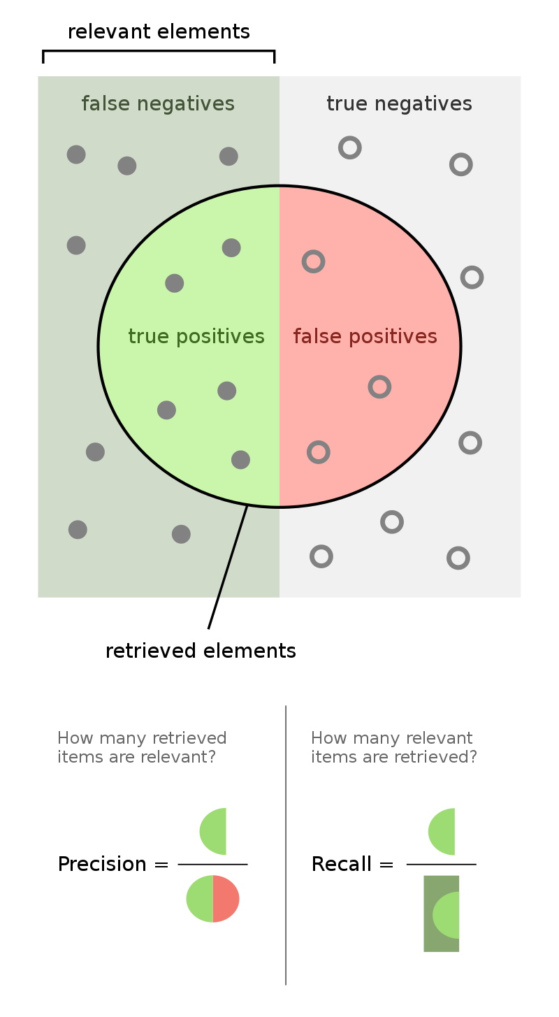
Recall
| Predicted Negative | Predicted Positive | |
|---|---|---|
| Actually Negative | TN = 90 ✅ | FP = 1 ❌ |
| Actually Positive | FN = 8 ❌ | TP = 1 ✅ |
🤔 Question: What proportion of individuals who actually have COVID did the test identify?
🙋 Answer: $\frac{1}{1 + 8} = \frac{1}{9} \approx 0.11$
More generally, the recall of a binary classifier is the proportion of actually positive instances that are correctly classified. We'd like this number to be as close to 1 (100%) as possible.
$$\text{recall} = \frac{TP}{\text{# actually positive}} = \frac{TP}{TP + FN}$$To compute recall, look at the bottom (positive) row of the above confusion matrix.
Recall isn't everything, either!
$$\text{recall} = \frac{TP}{TP + FN}$$🤔 Question: Can you design a "COVID test" with perfect recall?
🙋 Answer: Yes – just predict that everyone has COVID!
| Predicted Negative | Predicted Positive | |
|---|---|---|
| Actually Negative | TN = 0 ✅ | FP = 91 ❌ |
| Actually Positive | FN = 0 ❌ | TP = 9 ✅ |
Like accuracy, recall on its own is not a perfect metric. Even though the classifier we just created has perfect recall, it has 91 false positives!
Precision
| Predicted Negative | Predicted Positive | |
|---|---|---|
| Actually Negative | TN = 0 ✅ | FP = 91 ❌ |
| Actually Positive | FN = 0 ❌ | TP = 9 ✅ |
The precision of a binary classifier is the proportion of predicted positive instances that are correctly classified. We'd like this number to be as close to 1 (100%) as possible.
$$\text{precision} = \frac{TP}{\text{# predicted positive}} = \frac{TP}{TP + FP}$$To compute precision, look at the right (positive) column of the above confusion matrix.
Tip: A good way to remember the difference between precision and recall is that in the denominator for 🅿️recision, both terms have 🅿️ in them (TP and FP).
Note that the "everyone-has-COVID" classifier has perfect recall, but a precision of $\frac{9}{9 + 91} = 0.09$, which is quite low.
🚨 Key idea: There is a "tradeoff" between precision and recall. Ideally, you want both to be high. For a particular prediction task, one may be important than the other.
Precision and recall
$$\text{precision} = \frac{TP}{TP + FP} \: \: \: \: \: \: \: \: \text{recall} = \frac{TP}{TP + FN}$$🤔 Question: When might high precision be more important than high recall?
🙋 Answer: For instance, in deciding whether or not someone committed a crime. Here, false positives are really bad – they mean that an innocent person is charged!
🤔 Question: When might high recall be more important than high precision?
🙋 Answer: For instance, in medical tests. Here, false negatives are really bad – they mean that someone's disease goes undetected!
Discussion Question
Consider the confusion matrix shown below.
| Predicted Negative | Predicted Positive | |
|---|---|---|
| Actually Negative | TN = 22 ✅ | FP = 2 ❌ |
| Actually Positive | FN = 23 ❌ | TP = 18 ✅ |
What is the accuracy of the above classifier? The precision? The recall?
After calculating all three on your own, click below to see the answers.
👉 Accuracy
(22 + 18) / (22 + 2 + 23 + 18) = 40 / 65👉 Precision
18 / (18 + 2) = 9 / 10👉 Recall
18 / (18 + 23) = 18 / 41Example: Tumor malignancy prediction (via logistic regression)
Wisconsin breast cancer dataset
The Wisconsin breast cancer dataset (WBCD) is a commonly-used dataset for demonstrating binary classification. It is built into sklearn.datasets.
from sklearn.datasets import load_breast_cancer
loaded = load_breast_cancer() # explore the value of `loaded`!
data = loaded['data']
labels = 1 - loaded['target']
cols = loaded['feature_names']
bc = pd.DataFrame(data, columns=cols)
bc.head()
| mean radius | mean texture | mean perimeter | mean area | ... | worst concavity | worst concave points | worst symmetry | worst fractal dimension | |
|---|---|---|---|---|---|---|---|---|---|
| 0 | 17.990 | 10.380 | 122.800 | 1001.000 | ... | 0.712 | 0.265 | 0.460 | 0.119 |
| 1 | 20.570 | 17.770 | 132.900 | 1326.000 | ... | 0.242 | 0.186 | 0.275 | 0.089 |
| 2 | 19.690 | 21.250 | 130.000 | 1203.000 | ... | 0.450 | 0.243 | 0.361 | 0.088 |
| 3 | 11.420 | 20.380 | 77.580 | 386.100 | ... | 0.687 | 0.258 | 0.664 | 0.173 |
| 4 | 20.290 | 14.340 | 135.100 | 1297.000 | ... | 0.400 | 0.163 | 0.236 | 0.077 |
5 rows × 30 columns
1 stands for "malignant", i.e. cancerous, and 0 stands for "benign", i.e. safe.
labels[:5]
array([1, 1, 1, 1, 1])
pd.Series(labels).value_counts(normalize=True)
0   0.627
1   0.373
dtype: float64
Our goal is to use the features in bc to predict labels.
Aside: Logistic regression
Logistic regression is a linear classification technique that builds upon linear regression. It models the probability of belonging to class 1, given a feature vector:
$$P(y = 1 | \vec{x}) = \sigma (\underbrace{w_0 + w_1 x^{(1)} + w_2 x^{(2)} + ... + w_d x^{(d)}}_{\text{linear regression model}})$$Here, $\sigma(t) = \frac{1}{1 + e^{-t}}$ is the sigmoid function; its outputs are between 0 and 1 (which means they can be interpreted as probabilities).
🤔 Question: Suppose our logistic regression model predicts the probability that a tumor is malignant is 0.75. What class do we predict – malignant or benign? What if the predicted probability is 0.3?
🙋 Answer: We have to pick a threshold (e.g. 0.5)!
- If the predicted probability is above the threshold, we predict malignant (1).
- Otherwise, we predict benign (0).
- In practice, use CV to decide threshold.
Fitting a logistic regression model
from sklearn.model_selection import train_test_split
from sklearn.linear_model import LogisticRegression
X_train, X_test, y_train, y_test = train_test_split(bc, labels)
clf = LogisticRegression(max_iter=10000)
clf.fit(X_train, y_train)
LogisticRegression(max_iter=10000)
How did clf come up with 1s and 0s?
clf.predict(X_test)
array([0, 0, 1, ..., 1, 0, 0])
It turns out that the predicted labels come from applying a threshold of 0.5 to the predicted probabilities. We can access the predicted probabilities via the predict_proba method:
# [:, 1] refers to the predicted probabilities for class 1
clf.predict_proba(X_test)
array([[1.  , 0.  ],
       [1.  , 0.  ],
       [0.  , 1.  ],
       ...,
       [0.45, 0.55],
       [0.99, 0.01],
       [1.  , 0.  ]])
Note that our model still has $w^*$s:
clf.intercept_
array([-29.98])
clf.coef_
array([[-0.81, -0.26, 0.41, ..., 0.38, 0.51, 0.08]])
Evaluating our model
Let's see how well our model does on the test set.
from sklearn import metrics
y_pred = clf.predict(X_test)
metrics.accuracy_score(y_test, y_pred)
0.9440559440559441
metrics.precision_score(y_test, y_pred)
0.9245283018867925
metrics.recall_score(y_test, y_pred)
0.9245283018867925
Which metric is more important for this task – precision or recall?
metrics.confusion_matrix(y_test, y_pred)
array([[86,  4],
       [ 4, 49]])
from sklearn.metrics import ConfusionMatrixDisplay
ConfusionMatrixDisplay.from_estimator(clf, X_test, y_test);
plt.grid(False)

What if we choose a different threshold?
🤔 Question: Suppose we choose a threshold higher than 0.5. What will happen to our model's precision and recall?
🙋 Answer: Precision will increase, while recall will decrease*.
- If the "bar" is higher to predict 1, then we will have fewer false positives.
- The denominator in $\text{precision} = \frac{TP}{TP + FP}$ will get smaller, and so precision will increase.
- However, the number of false negatives will increase, as we are being more "strict" about what we classify as positive, and so $\text{recall} = \frac{TP}{TP + FN}$ will decrease.
- *It is possible for either or both to stay the same, if changing the threshold slightly (e.g. from 0.5 to 0.500001) doesn't change any predictions.
Similarly, if we decrease our threshold, our model's precision will decrease, while its recall will increase.
Trying several thresholds
The classification threshold is not actually a hyperparameter of LogisticRegression, because the threshold doesn't change the coefficients ($w^*$s) of the logistic regression model itself (see this article for more details).
- Still, the threshold affects our decision rule, so we can tune it using CV.
- It's also useful to plot how our metrics change as we change the threshold.
thresholds = np.arange(0, 1.01, 0.01)
precisions = np.array([])
recalls = np.array([])

for t in thresholds:
    y_pred = clf.predict_proba(X_test)[:, 1] >= t
    precisions = np.append(precisions, metrics.precision_score(y_test, y_pred))
    recalls = np.append(recalls, metrics.recall_score(y_test, y_pred))
Let's visualize the results in plotly, which is interactive.
px.line(x=thresholds, y=precisions,
        labels={'x': 'Threshold', 'y': 'Precision'}, title='Precision vs. Threshold', width=1000, height=600)
px.line(x=thresholds, y=recalls,
        labels={'x': 'Threshold', 'y': 'Recall'}, title='Recall vs. Threshold', width=1000, height=600)
px.line(x=recalls, y=precisions, hover_name=thresholds,
        labels={'x': 'Recall', 'y': 'Precision'}, title='Precision vs. Recall')
The above curve is called a precision-recall (or PR) curve.
🤔 Question: Based on the PR curve above, what threshold would you choose?
Combining precision and recall
If we care equally about a model's precision $PR$ and recall $RE$, we can combine the two using a single metric called the F1-score:
$$\text{F1-score} = \text{harmonic mean}(PR, RE) = 2\frac{PR \cdot RE}{PR + RE}$$pr = metrics.precision_score(y_test, clf.predict(X_test))
re = metrics.recall_score(y_test, clf.predict(X_test))
2 * pr * re / (pr + re)
0.9245283018867925
metrics.f1_score(y_test, clf.predict(X_test))
0.9245283018867925
Both F1-score and accuracy are overall measures of a binary classifier's performance. But remember, accuracy is misleading in the presence of class imbalance, and doesn't take into account the kinds of errors the classifier makes.
metrics.accuracy_score(y_test, clf.predict(X_test))
0.9440559440559441
Other evaluation metrics for binary classifiers
We just scratched the surface! This excellent table from Wikipedia summarizes the many other metrics that exist.
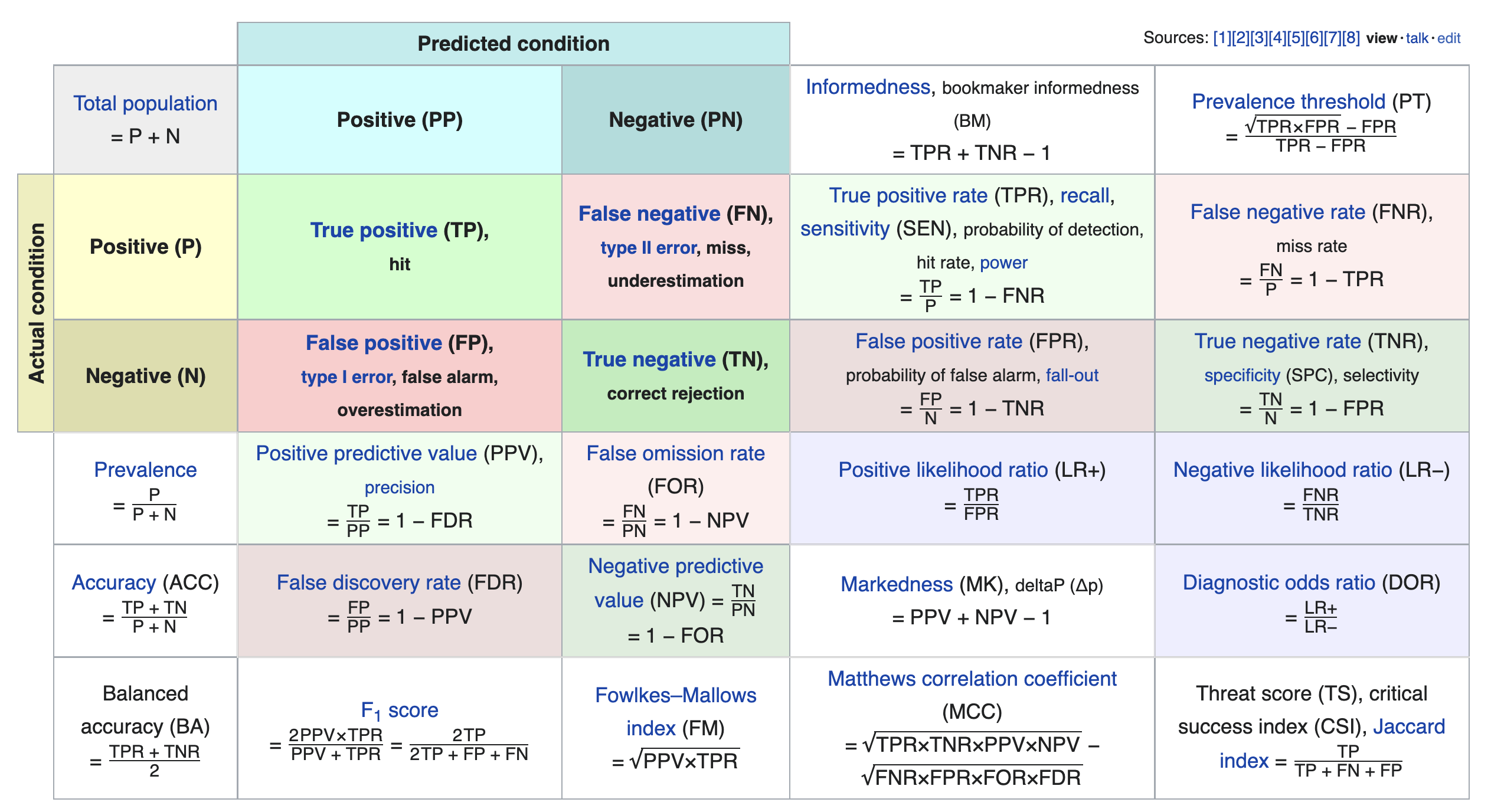
If you're interested in exploring further, a good next metric to look at is true negative rate (i.e. specificity), which is the analogue of recall for true negatives.