from dsc80_utils import *

Lecture 18 – Classifier Evaluation, Conclusion, Final Review

DSC 80, Fall 2023

📣 Announcements 📣

• Course evals (SET and End-of-Quarter Survey) due tomorrow at 11:59pm.
  • If 85% of class fills it out, everyone gets +1% to their final exam grade!
• Final Exam on Mon, Dec 11, 3-6pm in WLH 2005 (our usual lecture room).
• Final Project due Wed, Dec 13.
  • No slip days allowed, since we need to turn in grades right after it's due.

📝 Final Exam

• Monday, Dec 11, 3-6pm in WLH 2005 (usual lecture room).
  • Will write the exam to take about 2 hours, so you'll have a lot of time to double check your work.
• Two 8.5"x11" cheat sheets allowed of your own creation (handwritten on tablet, then printed is okay.)
• Covers every lecture, lab, and project.
• Similar format to the midterm: mix of fill-in-the-blank, multiple choice, and free response.
  • I use pandas fill-in-the-blank questions to test your ability to read and write code, not just write code from scratch, which is why they can feel tricker.
• Questions on final about pre-Midterm material will be marked as "M". Your Midterm grade will be the higher of your (z-score adjusted) grades on the Midterm and the questions marked as "M" on the final.

🙋🙋🏽‍♀️ Questions?

https://app.sli.do/event/2LZSnXWNpGPiuVnCZMa5J8

Example: Tumor malignancy prediction (via logistic regression)

Wisconsin breast cancer dataset

The Wisconsin breast cancer dataset (WBCD) is a commonly-used dataset for demonstrating binary classification. It is built into sklearn.datasets.

from sklearn.datasets import load_breast_cancer
loaded = load_breast_cancer() # explore the value of `loaded`!
data = loaded['data']
labels = 1 - loaded['target']
cols = loaded['feature_names']
bc = pd.DataFrame(data, columns=cols)

bc.head()

	mean radius	mean texture	mean perimeter	mean area	...	worst concavity	worst concave points	worst symmetry	worst fractal dimension
0	17.99	10.38	122.80	1001.0	...	0.71	0.27	0.46	0.12
1	20.57	17.77	132.90	1326.0	...	0.24	0.19	0.28	0.09
2	19.69	21.25	130.00	1203.0	...	0.45	0.24	0.36	0.09
3	11.42	20.38	77.58	386.1	...	0.69	0.26	0.66	0.17
4	20.29	14.34	135.10	1297.0	...	0.40	0.16	0.24	0.08

5 rows × 30 columns

1 stands for "malignant", i.e. cancerous, and 0 stands for "benign", i.e. safe.

labels[:5]

array([1, 1, 1, 1, 1])

pd.Series(labels).value_counts(normalize=True)

0    0.63
1    0.37
dtype: float64

Our goal is to use the features in bc to predict labels.

Aside: Logistic regression

Logistic regression is a linear classification technique that builds upon linear regression. It models the probability of belonging to class 1, given a feature vector:

$$P(y = 1 | \vec{x}) = \sigma (\underbrace{w_0 + w_1 x^{(1)} + w_2 x^{(2)} + ... + w_d x^{(d)}}_{\text{linear regression model}})$$

Here, $\sigma(t) = \frac{1}{1 + e^{-t}}$ is the sigmoid function; its outputs are between 0 and 1 (which means they can be interpreted as probabilities).

🤔 Question: Suppose our logistic regression model predicts the probability that a tumor is malignant is 0.75. What class do we predict – malignant or benign? What if the predicted probability is 0.3?

🙋 Answer: We have to pick a threshold (e.g. 0.5)!

• If the predicted probability is above the threshold, we predict malignant (1).
• Otherwise, we predict benign (0).
• In practice, use CV to decide threshold.

Fitting a logistic regression model

from sklearn.model_selection import train_test_split
from sklearn.linear_model import LogisticRegression

X_train, X_test, y_train, y_test = train_test_split(bc, labels)

clf = LogisticRegression(max_iter=10000)
clf.fit(X_train, y_train)

LogisticRegression(max_iter=10000)

How did clf come up with 1s and 0s?

clf.predict(X_test)

array([1, 1, 1, ..., 1, 0, 0])

It turns out that the predicted labels come from applying a threshold of 0.5 to the predicted probabilities. We can access the predicted probabilities via the predict_proba method:

# [:, 1] refers to the predicted probabilities for class 1
clf.predict_proba(X_test)

array([[0.02, 0.98],
       [0.  , 1.  ],
       [0.  , 1.  ],
       ...,
       [0.  , 1.  ],
       [0.91, 0.09],
       [1.  , 0.  ]])

Note that our model still has $w^*$s:

clf.intercept_

array([-26.93])

clf.coef_

array([[-1.04, -0.17,  0.19, ...,  0.48,  0.43,  0.1 ]])

Evaluating our model

Let's see how well our model does on the test set.

from sklearn import metrics

y_pred = clf.predict(X_test)

Which metric is more important for this task – precision or recall?

metrics.confusion_matrix(y_test, y_pred)

array([[87,  3],
       [ 5, 48]])

from sklearn.metrics import ConfusionMatrixDisplay
ConfusionMatrixDisplay.from_estimator(clf, X_test, y_test);
plt.grid(False)

metrics.accuracy_score(y_test, y_pred)

0.9440559440559441

metrics.precision_score(y_test, y_pred)

0.9411764705882353

metrics.recall_score(y_test, y_pred)

0.9056603773584906

What if we choose a different threshold?

🤔 Question: Suppose we choose a threshold higher than 0.5. What will happen to our model's precision and recall?

🙋 Answer: Precision will increase, while recall will decrease*.

• If the "bar" is higher to predict 1, then we will have fewer false positives.
• The denominator in $\text{precision} = \frac{TP}{TP + FP}$ will get smaller, and so precision will increase.
• However, the number of false negatives will increase, as we are being more "strict" about what we classify as positive, and so $\text{recall} = \frac{TP}{TP + FN}$ will decrease.
• *It is possible for either or both to stay the same, if changing the threshold slightly (e.g. from 0.5 to 0.500001) doesn't change any predictions.

Similarly, if we decrease our threshold, our model's precision will decrease, while its recall will increase.

Trying several thresholds

The classification threshold is not actually a hyperparameter of LogisticRegression, because the threshold doesn't change the coefficients ($w^*$s) of the logistic regression model itself (see this article for more details).

• Still, the threshold affects our decision rule, so we can tune it using CV.
• It's also useful to plot how our metrics change as we change the threshold.

thresholds = np.arange(0.01, 1.01, 0.01)
precisions = np.array([])
recalls = np.array([])

for t in thresholds:
    y_pred = clf.predict_proba(X_test)[:, 1] >= t
    precisions = np.append(precisions, metrics.precision_score(y_test, y_pred, zero_division=1))
    recalls = np.append(recalls, metrics.recall_score(y_test, y_pred))

Let's visualize the results in plotly, which is interactive.

px.line(x=thresholds, y=precisions,
        labels={'x': 'Threshold', 'y': 'Precision'}, title='Precision vs. Threshold', width=1000, height=600)

px.line(x=thresholds, y=recalls, 
        labels={'x': 'Threshold', 'y': 'Recall'}, title='Recall vs. Threshold', width=1000, height=600)

px.line(x=recalls, y=precisions, hover_name=thresholds, 
        labels={'x': 'Recall', 'y': 'Precision'}, title='Precision vs. Recall')

The above curve is called a precision-recall (or PR) curve.

🤔 Question: Based on the PR curve above, what threshold would you choose?

Combining precision and recall

If we care equally about a model's precision $PR$ and recall $RE$, we can combine the two using a single metric called the F1-score:

$$\text{F1-score} = \text{harmonic mean}(PR, RE) = 2\frac{PR \cdot RE}{PR + RE}$$

pr = metrics.precision_score(y_test, clf.predict(X_test))
re = metrics.recall_score(y_test, clf.predict(X_test))

2 * pr * re / (pr + re)

0.923076923076923

metrics.f1_score(y_test, clf.predict(X_test))

0.923076923076923

Both F1-score and accuracy are overall measures of a binary classifier's performance. But remember, accuracy is misleading in the presence of class imbalance, and doesn't take into account the kinds of errors the classifier makes.

metrics.accuracy_score(y_test, clf.predict(X_test))

0.9440559440559441

Other evaluation metrics for binary classifiers

We just scratched the surface! This excellent table from Wikipedia summarizes the many other metrics that exist.

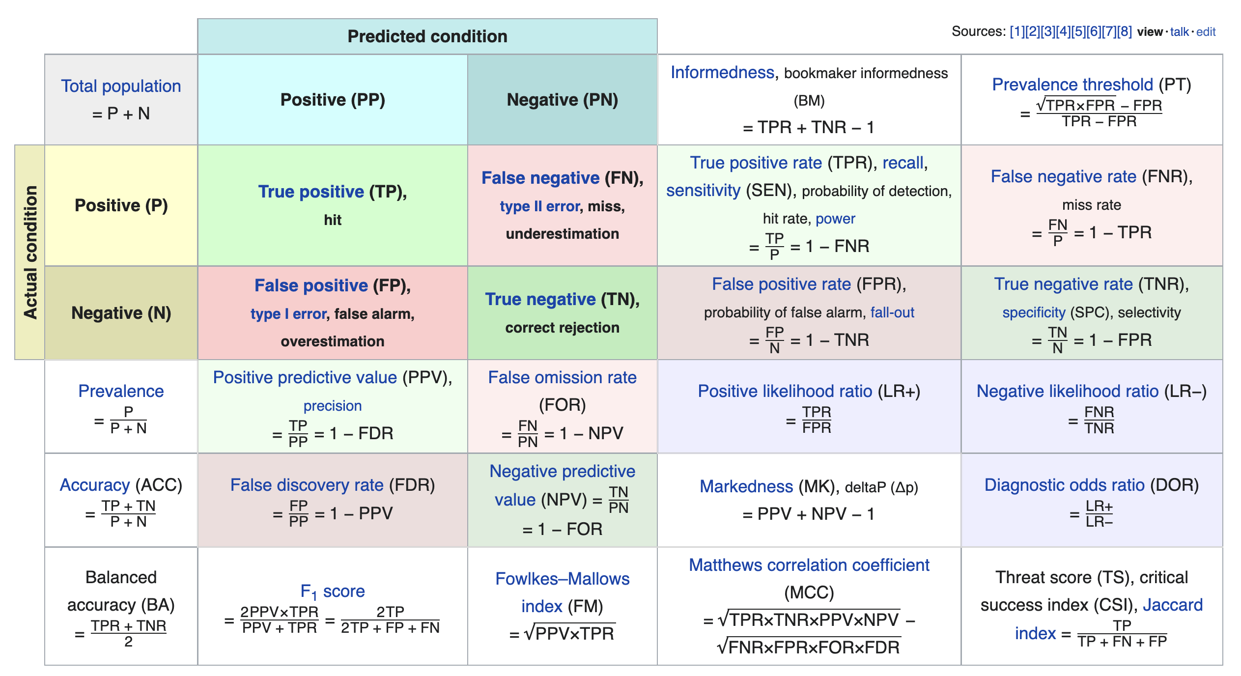
If you're interested in exploring further, a good next metric to look at is true negative rate (i.e. specificity), which is the analogue of recall for true negatives.

🙋🙋🏽‍♀️ Questions?

https://app.sli.do/event/2LZSnXWNpGPiuVnCZMa5J8

Parting thoughts

Course goals ✅

In this course, you...

• Practiced translating potentially vague questions into quantitative questions about measurable observations.
• Learned to reason about 'black-box' processes (e.g. complicated models).
• Understood computational and statistical implications of working with data.
• Learned to use real data tools (e.g. love the documentation!).
• Got a taste of the "life of a data scientist".

Course outcomes ✅

Now, you...

• Are prepared for internships and data science "take home" interviews!
• Are ready to create your own portfolio of personal projects.
• Have the background and maturity to succeed in the upper-division.

Topics covered ✅

We learnt a lot this quarter.

• Week 1: From BabyPandas to Pandas
• Week 2: DataFrames
• Week 3: Messy Data, Hypothesis Testing
• Week 4: Missing Values and Imputation
• Week 5: HTTP, Midterm Exam
• Week 6: Web Scraping, Regex
• Week 7: Text Features, Regression
• Week 8: Feature Engineering
• Week 9: Generalization, CV, Decision Trees
• Week 10: Random Forests, Classifier Evaluation
• Week 11: Final Exam

🛠️ Guide to doing independent work, getting research lab positions, internships, etc.

[I'll draw on tablet for this]

Thank you!

• This course would not have been possible without our 7 tutors and 2 TAs: Dylan Stockard, Giorgia Nicolaou, Gabriel Cha, Lauren (Luran) Zhang, John (Jiayu) Chen, Sunan Xu, Doris (Ge) Gao, Tiffany Yu, and Zelong Wang.

• Don't be a stranger – our contact information is at dsc80.com/staff!

  • This quarter's course website will remain online permanently at dsc-courses.github.io.

• Apply to be a tutor in the future! Learn more here.

Final Review

With the time we have left, I'll cover tricky questions from past exams, as well as questions you may have!

https://app.sli.do/event/2LZSnXWNpGPiuVnCZMa5J8

Good luck on the Final Exam, and enjoy your winter break! 🎉