import pandas as pd
import numpy as np

import matplotlib.pyplot as plt
plt.style.use('ggplot')
plt.rcParams['figure.figsize'] = (10, 5)
I co-direct the Laboratory for Mobile Sensing and Ubiquitous Computing (MOSAIC lab).
Bio: Ph.D. Cornell University (2017), M.S. University of Texas at Dallas (2012), B.S. Bangladesh University of Engineering and Technology (2009).
Research Interest: Mobile and ubiquitous computing, human health and behavior modeling with statistical signal processing and machine learning, novel on-body and off-body sensor development with embedded systems and applied physics.
In addition to the instructor, we have 7 tutors and 1 TA, who are here to help you in discussion, office hours, and on Ed:
TA:
Praveen Ravi Nair
Tutors:
Yuxin Guo, Weiyue Li, Aishani Mohapatra, Costin Smilovici, Yujia Wang, Tiffany Yu, Diego Zavalza
Learn more about them at dsc80.com/staff.
In DSC 10, we told you that data science is about drawing useful conclusions from data using computation.
In DSC 10, you:
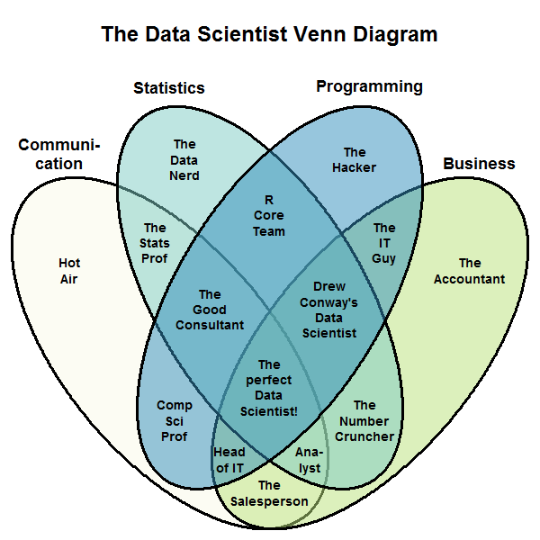
Let's look at a few more definitions of data science.
There isn't agreement on which "Venn Diagram" is correct!
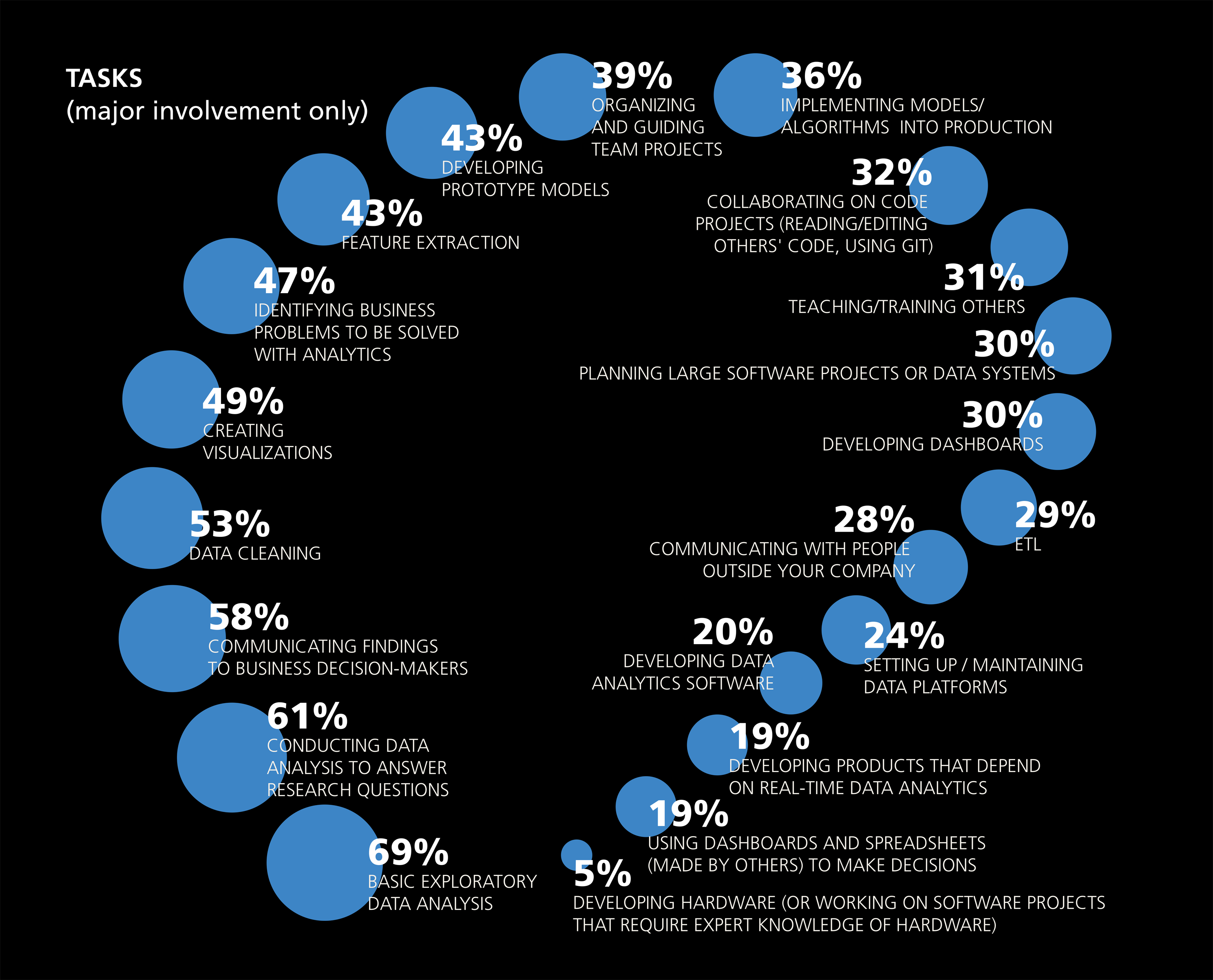
The chart below is taken from the 2016 Data Science Salary Survey, administered by O'Reilly. They asked respondents what they spend their time doing on a daily basis. What do you notice?
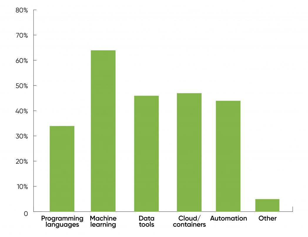
The chart below is taken from the followup 2021 Data/AI Salary Survey, also administered by O'Reilly. They asked respondents:
What technologies will have the biggest effect on compensation in the coming year?
My take: in DSC 80, and in the DSC major more broadly, we are training you to ask and answer questions using data.
As you take more courses, we're training you to answer questions whose answers are ambiguous – this uncertainly is what makes data science challenging!
Let's look at some examples of data science in practice.
Neuromophic High-Frequency 3D Dancing Pose Estimation in Dynamic Environment [https://www.youtube.com/watch?v=xmqMgzqAxIM].
OpiTrack:A Wearable-based Clinical Opioid Use Tracker with Temporal Convolutional Attention Networks [https://www.youtube.com/watch?v=zo2sz6DhK84]
MechanoBeat [https://www.youtube.com/watch?v=ZXA_eKm_bR8]
The decisions that we make as data scientists have the potential to impact the livelihoods of other people.
Good data analysis is not:
There are many tools out there for data science, but they are merely tools. They don’t do any of the important thinking – that's where you come in!
“The purpose of computing is insight, not numbers.” - R. Hamming. Numerical Methods for Scientists and Engineers (1962).
DSC 80 is about the practice of dealing with messy, ambiguous, and complex data.
In this course, you will...
After this course, you will...
This course was desgined by a former data scientist at Amazon (Aaron Fraenkel). As such, you'll be learning skills that you need to know as a data scientist.
babypandas to pandassklearn basicssklearn pipelines and model evaluationIn addition, you must fill out our Welcome Survey.
You will access all course content by pulling the course GitHub repository:
We will post HTML versions of lecture notebooks on the course website, but otherwise you must git pull from this repository to access all course materials (including blank copies of assignments).
In this course, you will learn by doing!
In DSC 80, assignments will usually consist of both a Jupyter Notebook and a .py file. You will write your code in the .py file; the Jupyter Notebook will contain problem descriptions and test cases. Lab 1 will explain the workflow.
In order to have you reflect on your lab work, we will offer extra credit each week if you do all 3 of the following:
Each week you do all 3, you'll earn 0.3% of extra credit – this could total 2.7%.
This scheme starts next week. Discussion will be podcasted.
| Sunday | Monday | Tuesday | Wednesday | Thursday | Friday | Saturday |
|---|---|---|---|---|---|---|
| Lecture | Lecture & Discussion | Lecture | ||||
| Lab due | Project/checkpoint due | Lab reflection due (extra credit) |
babypandas.It is no secret that this course requires a lot of work - becoming fluent with working with data is hard!
Once you've tried to solve problems on your own, we're glad to help.
You learned about the scientific method in elementary school.
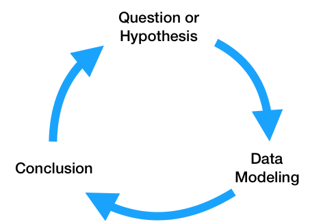
However, it hides a lot of complexity.
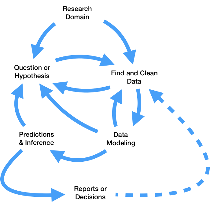
All steps lead to more questions! We'll refer back to the data science lifecycle repeatedly throughout the quarter.
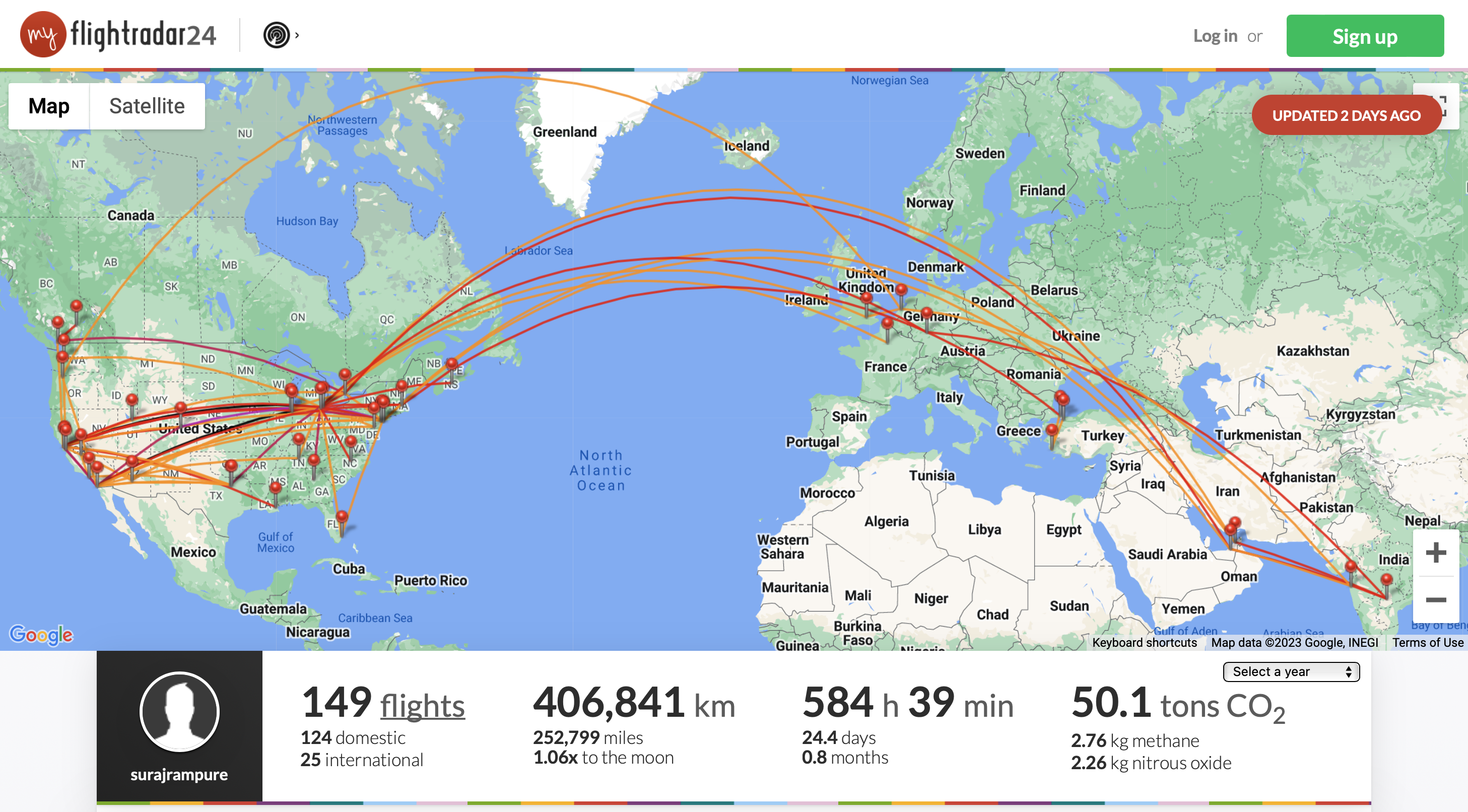
Goal: recreate this map.
myFlightradar24 is a free site that allows you to enter information about flights that you've been on and produces interesting visualizations using that information. The dataset we're working with is taken from my personal myFlightradar24 page, and contains every flight I've been on since 2014, plus some additional ones from years prior.
flights = pd.read_csv('data/flightdiary_2023_01_09_02_58.csv')
flights.head()
| Date | Flight number | From | To | Dep time | Arr time | Duration | Airline | Aircraft | Registration | Seat number | Seat type | Flight class | Flight reason | Note | Dep_id | Arr_id | Airline_id | Aircraft_id | |
|---|---|---|---|---|---|---|---|---|---|---|---|---|---|---|---|---|---|---|---|
| 0 | 2021-07-12 | AC8874 | Windsor / Windsor (YQG/CYQG) | Toronto / Pearson (YYZ/CYYZ) | 17:00:00 | 18:03:00 | 01:03:00 | Air Canada (AC/ACA) | Bombardier Dash 8-300 (DH8C) | C-GHTA | NaN | 3 | 1 | 1 | NaN | 3413 | 3500 | 13 | 609 |
| 1 | 2021-07-12 | AC127 | Toronto / Pearson (YYZ/CYYZ) | Vancouver / Vancouver (YVR/CYVR) | 19:00:00 | 20:46:00 | 04:46:00 | Air Canada (AC/ACA) | Boeing 787-9 (B789) | C-FRSR | NaN | 0 | 0 | 0 | NaN | 3500 | 3466 | 13 | 2088 |
| 2 | 2021-07-14 | 8P1205 | Vancouver / Vancouver (YVR/CYVR) | Kamloops / Kamloops (YKA/CYKA) | 14:35:00 | 15:25:00 | 00:50:00 | Pacific Coastal Airlines (8P/PCO) | Beechcraft 1900 (B190) | C-GPCL | NaN | 0 | 0 | 0 | NaN | 3466 | 3368 | 1011 | 189 |
| 3 | 2021-07-15 | 8P1206 | Kamloops / Kamloops (YKA/CYKA) | Vancouver / Vancouver (YVR/CYVR) | 15:50:00 | 16:40:00 | 00:50:00 | Pacific Coastal Airlines (8P/PCO) | Beechcraft 1900 (B190) | C-GPCE | NaN | 0 | 0 | 0 | NaN | 3368 | 3466 | 1011 | 189 |
| 4 | 2021-07-17 | AC114 | Vancouver / Vancouver (YVR/CYVR) | Toronto / Pearson (YYZ/CYYZ) | 11:30:00 | 18:50:00 | 04:20:00 | Air Canada (AC/ACA) | Boeing 777-300ER (B77W) | C-FIUV | NaN | 0 | 0 | 0 | NaN | 3466 | 3500 | 13 | 2023 |
flights.shape
(149, 19)
flights currently contains a lot of information that we're not going to use.
flights.head()
| Date | Flight number | From | To | Dep time | Arr time | Duration | Airline | Aircraft | Registration | Seat number | Seat type | Flight class | Flight reason | Note | Dep_id | Arr_id | Airline_id | Aircraft_id | |
|---|---|---|---|---|---|---|---|---|---|---|---|---|---|---|---|---|---|---|---|
| 0 | 2021-07-12 | AC8874 | Windsor / Windsor (YQG/CYQG) | Toronto / Pearson (YYZ/CYYZ) | 17:00:00 | 18:03:00 | 01:03:00 | Air Canada (AC/ACA) | Bombardier Dash 8-300 (DH8C) | C-GHTA | NaN | 3 | 1 | 1 | NaN | 3413 | 3500 | 13 | 609 |
| 1 | 2021-07-12 | AC127 | Toronto / Pearson (YYZ/CYYZ) | Vancouver / Vancouver (YVR/CYVR) | 19:00:00 | 20:46:00 | 04:46:00 | Air Canada (AC/ACA) | Boeing 787-9 (B789) | C-FRSR | NaN | 0 | 0 | 0 | NaN | 3500 | 3466 | 13 | 2088 |
| 2 | 2021-07-14 | 8P1205 | Vancouver / Vancouver (YVR/CYVR) | Kamloops / Kamloops (YKA/CYKA) | 14:35:00 | 15:25:00 | 00:50:00 | Pacific Coastal Airlines (8P/PCO) | Beechcraft 1900 (B190) | C-GPCL | NaN | 0 | 0 | 0 | NaN | 3466 | 3368 | 1011 | 189 |
| 3 | 2021-07-15 | 8P1206 | Kamloops / Kamloops (YKA/CYKA) | Vancouver / Vancouver (YVR/CYVR) | 15:50:00 | 16:40:00 | 00:50:00 | Pacific Coastal Airlines (8P/PCO) | Beechcraft 1900 (B190) | C-GPCE | NaN | 0 | 0 | 0 | NaN | 3368 | 3466 | 1011 | 189 |
| 4 | 2021-07-17 | AC114 | Vancouver / Vancouver (YVR/CYVR) | Toronto / Pearson (YYZ/CYYZ) | 11:30:00 | 18:50:00 | 04:20:00 | Air Canada (AC/ACA) | Boeing 777-300ER (B77W) | C-FIUV | NaN | 0 | 0 | 0 | NaN | 3466 | 3500 | 13 | 2023 |
flights = flights[['Date', 'Flight number', 'From', 'To', 'Airline']]
flights
| Date | Flight number | From | To | Airline | |
|---|---|---|---|---|---|
| 0 | 2021-07-12 | AC8874 | Windsor / Windsor (YQG/CYQG) | Toronto / Pearson (YYZ/CYYZ) | Air Canada (AC/ACA) |
| 1 | 2021-07-12 | AC127 | Toronto / Pearson (YYZ/CYYZ) | Vancouver / Vancouver (YVR/CYVR) | Air Canada (AC/ACA) |
| 2 | 2021-07-14 | 8P1205 | Vancouver / Vancouver (YVR/CYVR) | Kamloops / Kamloops (YKA/CYKA) | Pacific Coastal Airlines (8P/PCO) |
| 3 | 2021-07-15 | 8P1206 | Kamloops / Kamloops (YKA/CYKA) | Vancouver / Vancouver (YVR/CYVR) | Pacific Coastal Airlines (8P/PCO) |
| 4 | 2021-07-17 | AC114 | Vancouver / Vancouver (YVR/CYVR) | Toronto / Pearson (YYZ/CYYZ) | Air Canada (AC/ACA) |
| ... | ... | ... | ... | ... | ... |
| 144 | 2022-11-28 | DL179 | Amsterdam / Schiphol (AMS/EHAM) | Portland / Portland (PDX/KPDX) | Delta Air Lines (DL/DAL) |
| 145 | 2022-11-28 | AS724 | Portland / Portland (PDX/KPDX) | San Diego / San Diego International (SAN/KSAN) | Alaska Airlines (AS/ASA) |
| 146 | 2022-12-09 | DL934 | San Diego / San Diego International (SAN/KSAN) | Detroit / Detroit Metropolitan Wayne Co (DTW/K... | Delta Air Lines (DL/DAL) |
| 147 | 2023-01-06 | UA2681 | Detroit / Detroit Metropolitan Wayne Co (DTW/K... | Denver / Denver (DEN/KDEN) | United Airlines (UA/UAL) |
| 148 | 2023-01-06 | UA540 | Denver / Denver (DEN/KDEN) | San Diego / San Diego International (SAN/KSAN) | United Airlines (UA/UAL) |
149 rows × 5 columns
These three letter codes (e.g. 'SAN', 'JFK') are called "IATA codes." They're much more convenient to work with than say, 'San Diego / San Diego International (SAN/KSAN)'.
flights['From'].head(10)
0                         Windsor / Windsor (YQG/CYQG)
1                         Toronto / Pearson (YYZ/CYYZ)
2                     Vancouver / Vancouver (YVR/CYVR)
3                       Kamloops / Kamloops (YKA/CYKA)
4                     Vancouver / Vancouver (YVR/CYVR)
5                         Toronto / Pearson (YYZ/CYYZ)
6       San Diego / San Diego International (SAN/KSAN)
7    San Francisco / San Francisco International (S...
8    Detroit / Detroit Metropolitan Wayne Co (DTW/K...
9    Detroit / Detroit Metropolitan Wayne Co (DTW/K...
Name: From, dtype: object
Later this quarter, we'll learn how to perform this task in a more robust fashion, but for now, we can use Python string methods.
def extract_iata(full_name):
    start = full_name.index('(') + 1
    end = full_name.rfind('/')
    return full_name[start:end]
extract_iata('San Diego / San Diego International (SAN/KSAN)')
'SAN'
flights['From'] = flights['From'].apply(extract_iata)
flights['To'] = flights['To'].apply(extract_iata)
flights.head()
| Date | Flight number | From | To | Airline | |
|---|---|---|---|---|---|
| 0 | 2021-07-12 | AC8874 | YQG | YYZ | Air Canada (AC/ACA) |
| 1 | 2021-07-12 | AC127 | YYZ | YVR | Air Canada (AC/ACA) |
| 2 | 2021-07-14 | 8P1205 | YVR | YKA | Pacific Coastal Airlines (8P/PCO) |
| 3 | 2021-07-15 | 8P1206 | YKA | YVR | Pacific Coastal Airlines (8P/PCO) |
| 4 | 2021-07-17 | AC114 | YVR | YYZ | Air Canada (AC/ACA) |
The color of the line between a pair of airports is determined by how often one flew between that pair of airports. myFlightradar24 seems to use the following scheme:
counts = (flights
         .groupby(['From', 'To'])
         .count()
         .reset_index()
         .drop(columns=['Flight number', 'Airline'])
         .rename(columns={'Date': 'count'})
         .sort_values('count', ascending=False))

counts
| From | To | count | |
|---|---|---|---|
| 35 | DTW | SFO | 12 |
| 78 | SFO | DTW | 12 |
| 33 | DTW | SAN | 6 |
| 70 | SAN | DTW | 5 |
| 83 | SFO | SAN | 4 |
| ... | ... | ... | ... |
| 34 | DTW | SEA | 1 |
| 32 | DTW | RDU | 1 |
| 31 | DTW | ORD | 1 |
| 30 | DTW | MDW | 1 |
| 49 | JFK | AUH | 1 |
99 rows × 3 columns
Issue: This DataFrame counts (A, B) as being different than (B, A), though on the map these appear to be the same. How can we come up with a single row for every pair of airports, without using a for-loop?
homes = ['SAN', 'DTW']
counts[
    (counts['From'].isin(homes)) &
    (counts['To'].isin(homes))
]
| From | To | count | |
|---|---|---|---|
| 33 | DTW | SAN | 6 |
| 70 | SAN | DTW | 5 |
Suppose two IATA codes are 'XYZ' and 'ABC'. We can combine them to create a single string, by:
'-'.In this case, that yields 'ABC-XYZ'. If we do this for all rows in counts, we can then group by these new strings and construct one row per airport pair!
counts.head()
| From | To | count | |
|---|---|---|---|
| 35 | DTW | SFO | 12 |
| 78 | SFO | DTW | 12 |
| 33 | DTW | SAN | 6 |
| 70 | SAN | DTW | 5 |
| 83 | SFO | SAN | 4 |
def concatenate_iata(row):
    code1 = row['From']
    code2 = row['To']
    return '-'.join(np.sort([code1, code2]))

concatenate_iata(counts.iloc[1])
'DTW-SFO'
counts['Both'] = counts.apply(concatenate_iata, axis=1)
counts
| From | To | count | Both | |
|---|---|---|---|---|
| 35 | DTW | SFO | 12 | DTW-SFO |
| 78 | SFO | DTW | 12 | DTW-SFO |
| 33 | DTW | SAN | 6 | DTW-SAN |
| 70 | SAN | DTW | 5 | DTW-SAN |
| 83 | SFO | SAN | 4 | SAN-SFO |
| ... | ... | ... | ... | ... |
| 34 | DTW | SEA | 1 | DTW-SEA |
| 32 | DTW | RDU | 1 | DTW-RDU |
| 31 | DTW | ORD | 1 | DTW-ORD |
| 30 | DTW | MDW | 1 | DTW-MDW |
| 49 | JFK | AUH | 1 | AUH-JFK |
99 rows × 4 columns
both_counts = counts.groupby('Both').agg({'count': 'sum', 'From': np.min, 'To': np.max}).sort_values('count', ascending=False)
both_counts
| count | From | To | |
|---|---|---|---|
| Both | |||
| DTW-SFO | 24 | DTW | SFO |
| DTW-SAN | 11 | DTW | SAN |
| SAN-SFO | 6 | SAN | SFO |
| DTW-LGA | 6 | DTW | LGA |
| DEN-DTW | 5 | DEN | DTW |
| ... | ... | ... | ... |
| DTW-ORD | 1 | DTW | ORD |
| AMS-LHR | 1 | LHR | AMS |
| DTW-PHX | 1 | PHX | DTW |
| DTW-SEA | 1 | DTW | SEA |
| DTW-PHL | 1 | PHL | DTW |
68 rows × 3 columns
In order to draw a map, we need to know the position of each airport. Our dataset doesn't currently have that information, so we'll need to acquire it from somewhere else.
Fortunately, we have access to a CSV that contains this information!
airports = pd.read_csv('data/airports.csv')
airports.head()
| id | ident | type | name | latitude_deg | longitude_deg | elevation_ft | continent | iso_country | iso_region | municipality | scheduled_service | gps_code | iata_code | local_code | home_link | wikipedia_link | keywords | |
|---|---|---|---|---|---|---|---|---|---|---|---|---|---|---|---|---|---|---|
| 0 | 6523 | 00A | heliport | Total Rf Heliport | 40.070801 | -74.933601 | 11.0 | NaN | US | US-PA | Bensalem | no | 00A | NaN | 00A | NaN | NaN | NaN |
| 1 | 323361 | 00AA | small_airport | Aero B Ranch Airport | 38.704022 | -101.473911 | 3435.0 | NaN | US | US-KS | Leoti | no | 00AA | NaN | 00AA | NaN | NaN | NaN |
| 2 | 6524 | 00AK | small_airport | Lowell Field | 59.949200 | -151.695999 | 450.0 | NaN | US | US-AK | Anchor Point | no | 00AK | NaN | 00AK | NaN | NaN | NaN |
| 3 | 6525 | 00AL | small_airport | Epps Airpark | 34.864799 | -86.770302 | 820.0 | NaN | US | US-AL | Harvest | no | 00AL | NaN | 00AL | NaN | NaN | NaN |
| 4 | 6526 | 00AR | closed | Newport Hospital & Clinic Heliport | 35.608700 | -91.254898 | 237.0 | NaN | US | US-AR | Newport | no | NaN | NaN | NaN | NaN | NaN | 00AR |
Let's keep only the rows where the 'iata_code' is not missing, and only the relevant columns.
airports = airports.loc[airports['iata_code'].notnull(), ['iata_code', 'latitude_deg', 'longitude_deg']]
airports.head()
| iata_code | latitude_deg | longitude_deg | |
|---|---|---|---|
| 225 | UTK | 11.222000 | 169.852005 |
| 443 | OCA | 25.325399 | -80.274803 |
| 600 | PQS | 61.934601 | -162.899994 |
| 679 | CSE | 38.851918 | -106.928341 |
| 1096 | JCY | 30.251801 | -98.622498 |
There are two ways to combine the information in this DataFrame with both_counts:
merge the two DataFrames.'iata_code's to locations, and then use the dictionary to find the location of each airport given its 'iata_code'.Let's try the latter. To do so, we need to construct a dictionary with the required information.
iata_to_location = airports.set_index('iata_code').T.to_dict(orient='list')
iata_to_location['SAN']
/var/folders/y2/4f_dlpr94bvcxcm3tfvfl5fr0000gn/T/ipykernel_2052/2780243585.py:1: UserWarning: DataFrame columns are not unique, some columns will be omitted.
  iata_to_location = airports.set_index('iata_code').T.to_dict(orient='list')
[32.7336006165, -117.190002441]
both_counts.head()
| count | From | To | |
|---|---|---|---|
| Both | |||
| DTW-SFO | 24 | DTW | SFO |
| DTW-SAN | 11 | DTW | SAN |
| SAN-SFO | 6 | SAN | SFO |
| DTW-LGA | 6 | DTW | LGA |
| DEN-DTW | 5 | DEN | DTW |
both_counts['From loc'] = both_counts['From'].apply(lambda x: iata_to_location[x])
both_counts['Away loc'] = both_counts['To'].apply(lambda x: iata_to_location[x])
both_counts.head()
| count | From | To | From loc | Away loc | |
|---|---|---|---|---|---|
| Both | |||||
| DTW-SFO | 24 | DTW | SFO | [42.212398529052734, -83.35340118408203] | [37.61899948120117, -122.375] |
| DTW-SAN | 11 | DTW | SAN | [42.212398529052734, -83.35340118408203] | [32.7336006165, -117.190002441] |
| SAN-SFO | 6 | SAN | SFO | [32.7336006165, -117.190002441] | [37.61899948120117, -122.375] |
| DTW-LGA | 6 | DTW | LGA | [42.212398529052734, -83.35340118408203] | [40.777199, -73.872597] |
| DEN-DTW | 5 | DEN | DTW | [39.861698150635, -104.672996521] | [42.212398529052734, -83.35340118408203] |
We're getting closer...
We'll use the folium package to draw lines. It's not included in the dsc80 conda environment we're having you set up, so we must install it.
!pip install folium
Requirement already satisfied: folium in /Users/tauhidurrahman/opt/anaconda3/envs/dsc80/lib/python3.8/site-packages (0.14.0)
Requirement already satisfied: branca>=0.6.0 in /Users/tauhidurrahman/opt/anaconda3/envs/dsc80/lib/python3.8/site-packages (from folium) (0.6.0)
Requirement already satisfied: jinja2>=2.9 in /Users/tauhidurrahman/opt/anaconda3/envs/dsc80/lib/python3.8/site-packages (from folium) (3.1.2)
Requirement already satisfied: requests in /Users/tauhidurrahman/opt/anaconda3/envs/dsc80/lib/python3.8/site-packages (from folium) (2.26.0)
Requirement already satisfied: numpy in /Users/tauhidurrahman/opt/anaconda3/envs/dsc80/lib/python3.8/site-packages (from folium) (1.21.2)
Requirement already satisfied: MarkupSafe>=2.0 in /Users/tauhidurrahman/opt/anaconda3/envs/dsc80/lib/python3.8/site-packages (from jinja2>=2.9->folium) (2.1.2)
Requirement already satisfied: idna<4,>=2.5 in /Users/tauhidurrahman/opt/anaconda3/envs/dsc80/lib/python3.8/site-packages (from requests->folium) (3.4)
Requirement already satisfied: certifi>=2017.4.17 in /Users/tauhidurrahman/opt/anaconda3/envs/dsc80/lib/python3.8/site-packages (from requests->folium) (2022.12.7)
Requirement already satisfied: urllib3<1.27,>=1.21.1 in /Users/tauhidurrahman/opt/anaconda3/envs/dsc80/lib/python3.8/site-packages (from requests->folium) (1.26.7)
Requirement already satisfied: charset-normalizer~=2.0.0 in /Users/tauhidurrahman/opt/anaconda3/envs/dsc80/lib/python3.8/site-packages (from requests->folium) (2.0.12)
import folium
The core object in folium is the Map. To initialize one, it's a good idea to provide it a "center" – we can use the my hometown, on the eastern part of the continent.
flight_map = folium.Map(location=(42.317432, -83.026772), zoom_start=2, width='80%', height='60%')
flight_map
To draw a line between two points, we create folium.PolyLine object, and call the add_to method on it.
both_counts.head()
| count | From | To | From loc | Away loc | |
|---|---|---|---|---|---|
| Both | |||||
| DTW-SFO | 24 | DTW | SFO | [42.212398529052734, -83.35340118408203] | [37.61899948120117, -122.375] |
| DTW-SAN | 11 | DTW | SAN | [42.212398529052734, -83.35340118408203] | [32.7336006165, -117.190002441] |
| SAN-SFO | 6 | SAN | SFO | [32.7336006165, -117.190002441] | [37.61899948120117, -122.375] |
| DTW-LGA | 6 | DTW | LGA | [42.212398529052734, -83.35340118408203] | [40.777199, -73.872597] |
| DEN-DTW | 5 | DEN | DTW | [39.861698150635, -104.672996521] | [42.212398529052734, -83.35340118408203] |
folium.PolyLine(both_counts.iloc[0].loc['From loc':].values, color='purple').add_to(flight_map)
<folium.vector_layers.PolyLine at 0x7fda09050280>
flight_map
Great! Now we need to do this for all pairs of airports, and make sure the color of each line matches the frequency of the route.
We'll use the scheme mentioned earlier to determine the color of each line.
def compute_color(count):
    if count > np.percentile(both_counts['count'], 98):
        return 'black'
    elif count > np.percentile(both_counts['count'], 95):
        return 'purple'
    elif count > 1:
        return 'red'
    else:
        return 'orange'
Now, we'll create a folium.PolyLine for each pair in both_counts, setting the color appropriately.
both_counts.head()
| count | From | To | From loc | Away loc | |
|---|---|---|---|---|---|
| Both | |||||
| DTW-SFO | 24 | DTW | SFO | [42.212398529052734, -83.35340118408203] | [37.61899948120117, -122.375] |
| DTW-SAN | 11 | DTW | SAN | [42.212398529052734, -83.35340118408203] | [32.7336006165, -117.190002441] |
| SAN-SFO | 6 | SAN | SFO | [32.7336006165, -117.190002441] | [37.61899948120117, -122.375] |
| DTW-LGA | 6 | DTW | LGA | [42.212398529052734, -83.35340118408203] | [40.777199, -73.872597] |
| DEN-DTW | 5 | DEN | DTW | [39.861698150635, -104.672996521] | [42.212398529052734, -83.35340118408203] |
for route_str, row in both_counts.iterrows():
    route = [row['From loc'], row['Away loc']]
    color = compute_color(row['count'])
    folium.PolyLine(route, color=color).add_to(flight_map)
Let's see what we've produced!
flight_map
It's not perfect:
We don't have time to make these fixes now, but try making those changes yourself (and let us know how it goes)!
pandas.