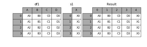
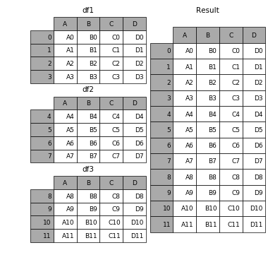
import pandas as pd
import numpy as np
import os

Lecture 6 – Concatenating and Merging

DSC 80, Spring 2023

Agenda

• Aside: Time series data.
• Concatenating DataFrames vertically and horizontally.
• Merging.
  • Types of joins.
  • Many-to-one and many-to-many joins.

Aside: Working with time series data

Time series – why now?

• We're about to start looking at how to combine multiple DataFrames.
• Data is often partitioned by time. For instance, there may be one .csv file per day for 1 year.
• We will need to load in the files as DataFrames and pd.concat them together.
• Note: "time series" is a general term and is not related to Series in pandas.

Datetime types

When working with time data, you will see two different kinds of "times":

• Datetimes reference particular moments in time (e.g. November 26th, 1998 at 8:26AM).
  • Could just be a date, e.g. January 23, 2023.
  • Could just be a time, e.g. 4:45 AM.
  • Datetimes typically don't keep track of timezones.

• Timedeltas, or durations, reference an exact length of time (e.g. a duration of 3 hours).

The datetime module

Python has an in-built datetime module, which contains datetime and timedelta types. These are much more convenient to deal with than strings that contain times.

import datetime

datetime.datetime.now()

datetime.datetime(2023, 4, 17, 11, 9, 18, 724440)

datetime.datetime.now() + datetime.timedelta(days=3, hours=5)

datetime.datetime(2023, 4, 20, 16, 9, 18, 730890)

Unix timestamps count the number of seconds since January 1st, 1970.

datetime.datetime.now().timestamp()

1681754958.73377

Times in pandas

• pd.Timestamp is the pandas equivalent of datetime.
• pd.to_datetime converts strings to pd.Timestamp objects.

pd.Timestamp(year=1998, month=11, day=26)

Timestamp('1998-11-26 00:00:00')

final_start = pd.to_datetime('14th June, 2023, 11:30AM')
final_start

Timestamp('2023-06-14 11:30:00')

final_finish = pd.to_datetime('June 14th, 2023, 2:30PM')
final_finish

Timestamp('2023-06-14 14:30:00')

Timestamps have time-related attributes, e.g. dayofweek, hour, min, sec.

# 0 is Monday, 1 is Tuesday, etc.
final_finish.dayofweek

2

final_finish.hour

14

Subtracting timestamps yields pd.Timedelta objects.

final_finish - final_start

Timedelta('0 days 03:00:00')

Example: Exam speeds

Below, we have the Final Exam starting and ending times for two sections of a course.

exam_times = pd.read_csv(os.path.join('data', 'exam-times.csv'))
exam_times

	name	start_exam	finish_exam	section
0	Annie	15:00	16:00	A
1	Billy	15:02	17:58	A
2	Sally	15:01	17:05	A
3	Tommy	15:00	16:55	A
4	Junior	18:00	20:00	B
5	Rex	18:06	20:50	B
6	Flash	19:07	20:59	B

Question: Who took the longest time to finish the exam?

# Step 1: Convert the time columns to timestamps, using pd.to_datetime.
exam_times['start_exam'] = pd.to_datetime(exam_times['start_exam'])
exam_times['finish_exam'] = pd.to_datetime(exam_times['finish_exam'])
exam_times

	name	start_exam	finish_exam	section
0	Annie	2023-04-17 15:00:00	2023-04-17 16:00:00	A
1	Billy	2023-04-17 15:02:00	2023-04-17 17:58:00	A
2	Sally	2023-04-17 15:01:00	2023-04-17 17:05:00	A
3	Tommy	2023-04-17 15:00:00	2023-04-17 16:55:00	A
4	Junior	2023-04-17 18:00:00	2023-04-17 20:00:00	B
5	Rex	2023-04-17 18:06:00	2023-04-17 20:50:00	B
6	Flash	2023-04-17 19:07:00	2023-04-17 20:59:00	B

# Note that datetime64[ns] is the data type pandas uses to store timestamps in a Series/DataFrame.
exam_times.dtypes

name                   object
start_exam     datetime64[ns]
finish_exam    datetime64[ns]
section                object
dtype: object

# Step 2: Find the difference between the two time columns.
exam_times['difference'] = exam_times['finish_exam'] - exam_times['start_exam']
exam_times

	name	start_exam	finish_exam	section	difference
0	Annie	2023-04-17 15:00:00	2023-04-17 16:00:00	A	0 days 01:00:00
1	Billy	2023-04-17 15:02:00	2023-04-17 17:58:00	A	0 days 02:56:00
2	Sally	2023-04-17 15:01:00	2023-04-17 17:05:00	A	0 days 02:04:00
3	Tommy	2023-04-17 15:00:00	2023-04-17 16:55:00	A	0 days 01:55:00
4	Junior	2023-04-17 18:00:00	2023-04-17 20:00:00	B	0 days 02:00:00
5	Rex	2023-04-17 18:06:00	2023-04-17 20:50:00	B	0 days 02:44:00
6	Flash	2023-04-17 19:07:00	2023-04-17 20:59:00	B	0 days 01:52:00

exam_times.dtypes

name                    object
start_exam      datetime64[ns]
finish_exam     datetime64[ns]
section                 object
difference     timedelta64[ns]
dtype: object

# Step 3: Sort by the difference in descending order and take the first row.
exam_times.sort_values('difference', ascending=False)['name'].iloc[0]

'Billy'

Concatenating vertically

# Run this cell to set up the next example.

section_A = pd.DataFrame({
    'Name': ['Annie', 'Billy', 'Sally', 'Tommy'],
    'Midterm': [98, 82, 23, 45],
    'Final': [88, 100, 99, 67]
})

section_B = pd.DataFrame({
    'Name': ['Junior', 'Rex', 'Flash'],
    'Midterm': [70, 99, 81],
    'Final': [42, 25, 90]
})

section_C = pd.DataFrame({
    'Name': ['Justin', 'Marina'],
    'Final': [98, 52]
})

section_D = pd.DataFrame({
    'Midterm': [10, 30, 80],
    'Name': ['Janine', 'Sooh', 'Suraj']
})

Example: Grades

Consider the students from our previous example. Suppose their grades are given to us in separate DataFrames. Note that these DataFrames contain the same attributes, but for different individuals.

section_A

	Name	Midterm	Final
0	Annie	98	88
1	Billy	82	100
2	Sally	23	99
3	Tommy	45	67

section_B

	Name	Midterm	Final
0	Junior	70	42
1	Rex	99	25
2	Flash	81	90

Question: How do we combine both DataFrames into a single, larger DataFrame?

Concatenating vertically

• The pd.concat function combines DataFrame and Series objects.
• By default, the rows of objects are stacked on top of one another.
• pd.concat has many options; we'll learn some of them here, and you'll discover the others by reading the documentation.

Example: Grades

By default, pd.concat takes a list of DataFrames and stacks them row-wise, i.e. on top of one another.

section_A

	Name	Midterm	Final
0	Annie	98	88
1	Billy	82	100
2	Sally	23	99
3	Tommy	45	67

section_B

	Name	Midterm	Final
0	Junior	70	42
1	Rex	99	25
2	Flash	81	90

pd.concat([section_A, section_B])

	Name	Midterm	Final
0	Annie	98	88
1	Billy	82	100
2	Sally	23	99
3	Tommy	45	67
0	Junior	70	42
1	Rex	99	25
2	Flash	81	90

Setting the optional argument ignore_index to True fixes the index (which .reset_index() also could do).

pd.concat([section_A, section_B], ignore_index=True)

	Name	Midterm	Final
0	Annie	98	88
1	Billy	82	100
2	Sally	23	99
3	Tommy	45	67
4	Junior	70	42
5	Rex	99	25
6	Flash	81	90

To keep track of which original DataFrame each row came from, we can use the keys optional argument, though if we do this, the resulting DataFrame has a MultiIndex.

combined = pd.concat([section_A, section_B], keys=['Section A', 'Section B'])
combined

		Name	Midterm	Final
Section A	0	Annie	98	88
	1	Billy	82	100
	2	Sally	23	99
	3	Tommy	45	67
Section B	0	Junior	70	42
	1	Rex	99	25
	2	Flash	81	90

combined.loc['Section A']

	Name	Midterm	Final
0	Annie	98	88
1	Billy	82	100
2	Sally	23	99
3	Tommy	45	67

Adding a single row

To add a single row to a DataFrame, create a new DataFrame that contains the single row, and use pd.concat.

The DataFrame append method does exist, though it's deprecated.

new_row_data = {'Name': 'King Triton', 'Midterm': 21, 'Final': 94}
new_row_df = pd.DataFrame([new_row_data]) # Note the list!
new_row_df

	Name	Midterm	Final
0	King Triton	21	94

pd.concat([section_A, new_row_df])

	Name	Midterm	Final
0	Annie	98	88
1	Billy	82	100
2	Sally	23	99
3	Tommy	45	67
0	King Triton	21	94

Missing columns?

If we concatenate two DataFrames that don't share the same column names, NaNs are added in the columns that aren't shared.

section_C

	Name	Final
0	Justin	98
1	Marina	52

section_D

	Midterm	Name
0	10	Janine
1	30	Sooh
2	80	Suraj

# Note that the 'Name' columns were combined, despite not being in the same position!
pd.concat([section_C, section_D])

	Name	Final	Midterm
0	Justin	98.0	NaN
1	Marina	52.0	NaN
0	Janine	NaN	10.0
1	Sooh	NaN	30.0
2	Suraj	NaN	80.0

⚠️ Warning: No loops!

• pd.concat returns a copy; it does not modify any of the input DataFrames.
• Do not use pd.concat in a loop, as it has terrible time and space efficiency.

total = pd.DataFrame()
for df in dataframes:
    total = total.concat(df)

• Instead, use pd.concat(dataframes), where dataframes is a list of DataFrames.

Aside: Accessing file names programmatically

• At times, you'll need to load in all of the files in a given folder.
• os.listdir(dirname) returns a list of the names of the files in the folder dirname.

import os
os.listdir('data')

['exam-times.csv']

os.listdir('../')

['lec22',
 'lec25',
 'lec13',
 'lec14',
 'lec15',
 'lec12',
 'lec24',
 'lec23',
 '.DS_Store',
 'lec01',
 'lec06',
 'lec08',
 'lec09',
 'lec07',
 'lec19',
 'lec26',
 'lec21',
 'lec17',
 'lec10',
 'lec11',
 'lec16',
 'lec20',
 'lec18',
 'lec27',
 'lec05',
 'lec02',
 'lec03',
 'lec04']

The following does something similar, but in the shell.

!ls ../

lec01 lec04 lec07 lec10 lec13 lec16 lec19 lec22 lec25
lec02 lec05 lec08 lec11 lec14 lec17 lec20 lec23 lec26
lec03 lec06 lec09 lec12 lec15 lec18 lec21 lec24 lec27

Concatenating horizontally

# Run this cell to set up the next example.

exams = section_A.copy()

assignments = exams[['Name']].assign(Homeworks=[99, 45, 23, 81],
                                     Labs=[100, 100, 99, 100])

overall = pd.DataFrame({
    'PID': ['A15253545', 'A10348245', 'A13349069', 'A18485824', 'A10094857'],
    'Student': ['Billy', 'Sally', 'Annie', 'Larry', 'Johnny'],
    'Final': [88, 64, 91, 45, 89]
})

Example: Grades (again)

Suppose we have two DataFrames, exams and assignments, which both contain different attributes for the same individuals.

exams

	Name	Midterm	Final
0	Annie	98	88
1	Billy	82	100
2	Sally	23	99
3	Tommy	45	67

assignments

	Name	Homeworks	Labs
0	Annie	99	100
1	Billy	45	100
2	Sally	23	99
3	Tommy	81	100

If we try to combine these DataFrames with pd.concat, we don't quite get what we're looking for.

pd.concat([exams, assignments])

	Name	Midterm	Final	Homeworks	Labs
0	Annie	98.0	88.0	NaN	NaN
1	Billy	82.0	100.0	NaN	NaN
2	Sally	23.0	99.0	NaN	NaN
3	Tommy	45.0	67.0	NaN	NaN
0	Annie	NaN	NaN	99.0	100.0
1	Billy	NaN	NaN	45.0	100.0
2	Sally	NaN	NaN	23.0	99.0
3	Tommy	NaN	NaN	81.0	100.0

But that's where the axis argument becomes handy.

Remember, most pandas operations default to axis=0, but here we want to concatenate the columns of exams to the columns of assignments, so we should use axis=1.

pd.concat([exams, assignments], axis=1)

	Name	Midterm	Final	Name	Homeworks	Labs
0	Annie	98	88	Annie	99	100
1	Billy	82	100	Billy	45	100
2	Sally	23	99	Sally	23	99
3	Tommy	45	67	Tommy	81	100

Note that the 'Name' column appears twice!

Concatenating horizontally

• To concatenate two DataFrames horizontally, use pd.concat with axis=1.
• Concatenation is done by matching indexes, regardless of their order. It does not look at the information in any of the columns!

Note that the call to pd.concat below combines information about each individual correctly, even though the orders of the names in exams_by_name and assignments_by_name are different.

# .loc[::-1] reverses the rows of the DataFrame.
exams_by_name = exams.set_index('Name').iloc[::-1]
exams_by_name

	Midterm	Final
Name
Tommy	45	67
Sally	23	99
Billy	82	100
Annie	98	88

assignments_by_name = assignments.set_index('Name')
assignments_by_name

	Homeworks	Labs
Name
Annie	99	100
Billy	45	100
Sally	23	99
Tommy	81	100

pd.concat([exams_by_name, assignments_by_name], axis=1)

	Midterm	Final	Homeworks	Labs
Name
Tommy	45	67	81	100
Sally	23	99	23	99
Billy	82	100	45	100
Annie	98	88	99	100

Remember that pd.concat only looks at the index when combining rows, not at any other columns.

exams_reversed = exams.iloc[::-1].reset_index(drop=True)
exams_reversed

	Name	Midterm	Final
0	Tommy	45	67
1	Sally	23	99
2	Billy	82	100
3	Annie	98	88

assignments

	Name	Homeworks	Labs
0	Annie	99	100
1	Billy	45	100
2	Sally	23	99
3	Tommy	81	100

pd.concat([exams_reversed, assignments], axis=1)

	Name	Midterm	Final	Name	Homeworks	Labs
0	Tommy	45	67	Annie	99	100
1	Sally	23	99	Billy	45	100
2	Billy	82	100	Sally	23	99
3	Annie	98	88	Tommy	81	100

Summary: pd.concat

• pd.concat "stitches" two or more DataFrames together.
• If you use axis=0, the DataFrames are concatenated vertically based on column names (rows on top of rows).
• If you use axis=1, the DataFrames are concatenated horizontally based on row indexes (columns next to columns).

Merging

Joining

• pd.concat with axis=1 combines DataFrames horizontally.
• To combine the rows of DataFrames in more advanced ways, we perform a join (SQL term), i.e. a merge (pandas term).
• A join is appropriate when we have two sources of information about the same individuals that is linked by a common column.
• The common column is called the join key.

# Run these two cells to set up the next example.

temps = pd.DataFrame({
    'City': ['San Diego', 'Toronto', 'Rome'],
    'Temperature': [76, 28, 56]
})

countries = pd.DataFrame({
    'City': ['Toronto', 'Shanghai', 'San Diego'],
    'Country': ['Canada', 'China', 'USA']
})

%reload_ext pandas_tutor

Let's work with a small example.

temps

	City	Temperature
0	San Diego	76
1	Toronto	28
2	Rome	56

countries

	City	Country
0	Toronto	Canada
1	Shanghai	China
2	San Diego	USA

temps_city = temps.set_index('City')
temps_city

	Temperature
City
San Diego	76
Toronto	28
Rome	56

countries_city = countries.set_index('City')
countries_city

	Country
City
Toronto	Canada
Shanghai	China
San Diego	USA

pd.concat([temps_city, countries_city],axis=1)

	Temperature	Country
City
San Diego	76.0	USA
Toronto	28.0	Canada
Rome	56.0	NaN
Shanghai	NaN	China

We'd like to combine both DataFrames, but it's not immediately clear if pd.concat would be useful.

It turns out that the right tool to use is the merge method.

%%pt

temps.merge(countries)

The merge method

• The merge DataFrame method joins two tables by columns or indexes.
  • "Merge" is just pandas' word for "join".

• When using the merge method, the DataFrame before .merge is the "left" DataFrame, and the DataFrame passed into .merge is the "right" DataFrame.
  • In temps.merge(countries), temps is considered the "left" DataFrame and countries is the "right" DataFrame; the columns from the left DataFrame appear to the left of the columns from right DataFrame.

• By default:
  • If join keys are not specified, all shared columns between the two DataFrames are used.
  • The "type" of join performed is an inner join.

Join types: inner joins

• Note that 'Rome' and 'Shanghai' do not appear in the merged DataFrame.
• This is because there is:
  • no city named 'Rome' in the right DataFrame, and
  • no city named 'Shanghai' in the left DataFrame.
• The default type of join that merge performs is an inner join, which keeps the intersection of the join keys.

Different join types

We can change the type of join performed by changing the how argument in merge. Let's experiment!

temps

	City	Temperature
0	San Diego	76
1	Toronto	28
2	Rome	56

countries

	City	Country
0	Toronto	Canada
1	Shanghai	China
2	San Diego	USA

# The default value of how is 'inner'.
temps.merge(countries, how='inner')

	City	Temperature	Country
0	San Diego	76	USA
1	Toronto	28	Canada

# Note the NaNs!
temps.merge(countries, how='left')

	City	Temperature	Country
0	San Diego	76	USA
1	Toronto	28	Canada
2	Rome	56	NaN

temps.merge(countries, how='right')

	City	Temperature	Country
0	Toronto	28.0	Canada
1	Shanghai	NaN	China
2	San Diego	76.0	USA

%%pt

temps.merge(countries, how='outer')

Note that an outer join is what pd.concat performs by default, when there are no duplicated keys in either DataFrame.

pd.concat([temps.set_index('City'), countries.set_index('City')], axis=1)

	Temperature	Country
City
San Diego	76.0	USA
Toronto	28.0	Canada
Rome	56.0	NaN
Shanghai	NaN	China

Different join types handle mismatches differently

There are four types of joins.

• Inner: keep only matching keys (intersection).
• Outer: keeps all keys in both DataFrames (union).
• Left: keep all keys in the left DataFrame, whether or not they are in the right DataFrame.
• Right: keep all keys in the right DataFrame, whether or not they are in the left DataFrame.

Symmetry

Note that a.merge(b, how='left') contains the same information as b.merge(a, how='right'), just in a different order.

temps.merge(countries, how='left')

	City	Temperature	Country
0	San Diego	76	USA
1	Toronto	28	Canada
2	Rome	56	NaN

countries.merge(temps, how='right')

	City	Country	Temperature
0	San Diego	USA	76
1	Toronto	Canada	28
2	Rome	NaN	56

Specifying join keys

• pandas defaults to using all shared column names as join keys.
• If there are multiple shared column names and you only want to join on one of them, or if there are no shared column names, then you will need to specify which columns to join on.
• Two solutions:
  1. Use the on argument if the desired columns have the same names in both DataFrames.
  2. Use the left_on or left_index argument AND the right_on or right_index argument.

exams

	Name	Midterm	Final
0	Annie	98	88
1	Billy	82	100
2	Sally	23	99
3	Tommy	45	67

overall

	PID	Student	Final
0	A15253545	Billy	88
1	A10348245	Sally	64
2	A13349069	Annie	91
3	A18485824	Larry	45
4	A10094857	Johnny	89

This is not what we're looking for:

exams.merge(overall)

	Name	Midterm	Final	PID	Student
0	Annie	98	88	A15253545	Billy

Instead, we need to tell pandas to look in the 'Name' column of exams and 'Student' column of overall.

exams.merge(overall, left_on='Name', right_on='Student')

	Name	Midterm	Final_x	PID	Student	Final_y
0	Annie	98	88	A13349069	Annie	91
1	Billy	82	100	A15253545	Billy	88
2	Sally	23	99	A10348245	Sally	64

If there are shared column names in the two DataFrames you are merging that you are not using as join keys, '_x' and '_y' are appended to their names by default.

exams.merge(overall, left_on='Name', right_on='Student', suffixes=('_Exam', '_Overall'))

	Name	Midterm	Final_Exam	PID	Student	Final_Overall
0	Annie	98	88	A13349069	Annie	91
1	Billy	82	100	A15253545	Billy	88
2	Sally	23	99	A10348245	Sally	64

Many-to-one & many-to-many joins

One-to-one joins

• So far in this lecture, the joins we have worked with are called one-to-one joins.
• Neither the left DataFrame nor the right DataFrame contained any duplicates in the join key.
• What if there are duplicated join keys, in one or both of the DataFrames we are merging?

# Run this cell to set up the next example.

profs = pd.DataFrame(
[['Brad', 'UCB', 9],
 ['Janine', 'UCSD', 8],
 ['Marina', 'UIC', 7],
 ['Justin', 'OSU', 5],
 ['Soohyun', 'UCSD', 2],
 ['Suraj', 'UCB', 2]],
    columns=['Name', 'School', 'Years']
)

schools = pd.DataFrame({
    'Abr': ['UCSD', 'UCLA', 'UCB', 'UIC'],
    'Full': ['University of California, San Diego', 'University of California, Los Angeles', 'University of California, Berkeley', 'University of Illinois Chicago']
})

programs = pd.DataFrame({
    'uni': ['UCSD', 'UCSD', 'UCSD', 'UCB', 'OSU', 'OSU'],
    'dept': ['Math', 'HDSI', 'COGS', 'CS', 'Math', 'CS'],
    'grad_students': [205, 54, 281, 439, 304, 193]
})

Many-to-one joins

• Many-to-one joins are joins where one of the DataFrames contains duplicate values in the join key.
• The resulting DataFrame will preserve those duplicate entries as appropriate.

profs

	Name	School	Years
0	Brad	UCB	9
1	Janine	UCSD	8
2	Marina	UIC	7
3	Justin	OSU	5
4	Soohyun	UCSD	2
5	Suraj	UCB	2

schools

	Abr	Full
0	UCSD	University of California, San Diego
1	UCLA	University of California, Los Angeles
2	UCB	University of California, Berkeley
3	UIC	University of Illinois Chicago

Note that when merging profs and schools, the information from schools is duplicated.

• 'University of California, San Diego' appears twice.
• 'University of California, Berkeley' appears three times.

# Why is a left merge most appropriate here?
profs.merge(schools, left_on='School', right_on='Abr', how='left')

	Name	School	Years	Abr	Full
0	Brad	UCB	9	UCB	University of California, Berkeley
1	Janine	UCSD	8	UCSD	University of California, San Diego
2	Marina	UIC	7	UIC	University of Illinois Chicago
3	Justin	OSU	5	NaN	NaN
4	Soohyun	UCSD	2	UCSD	University of California, San Diego
5	Suraj	UCB	2	UCB	University of California, Berkeley

Many-to-many joins

Many-to-many joins are joins where both DataFrames have duplicate values in the join key.

profs

	Name	School	Years
0	Brad	UCB	9
1	Janine	UCSD	8
2	Marina	UIC	7
3	Justin	OSU	5
4	Soohyun	UCSD	2
5	Suraj	UCB	2

programs

	uni	dept	grad_students
0	UCSD	Math	205
1	UCSD	HDSI	54
2	UCSD	COGS	281
3	UCB	CS	439
4	OSU	Math	304
5	OSU	CS	193

Before running the following cell, try predicting the number of rows in the output.

%%pt

profs.merge(programs, left_on='School', right_on='uni')

• merge stitched together every UCSD row in profs with every UCSD row in programs.
• Since there were 2 UCSD rows in profs and 3 in programs, there are $2 \cdot 3 = 6$ UCSD rows in the output. The same applies for all other schools.

Summary, next time

Summary

• Timestamps in pandas are stored using pd.Timestamp and pd.Timedelta objects.
• pd.concat "stitches" two or more DataFrames together, either vertically or horizontally.
  • Vertically: looks at column names. Horizontally: looks at row indexes.
• The merge DataFrame method joins two DataFrames together based on a shared column, called a join key. There are four types of joins:
  • Inner join: keeps the intersection of the join keys.
  • Outer join: keeps the union of the join keys.
  • Left/right joins: keeps all of the join keys in the left/right DataFrame.
  • In outer/left/right joins, all missing fields are filled with NaNs.

Next time

Cleaning messy, real-world data.