In [1]:
import pandas as pd
import numpy as np
import os

import plotly.express as px
import plotly.graph_objects as go
pd.options.plotting.backend = 'plotly'
TEMPLATE = 'seaborn'
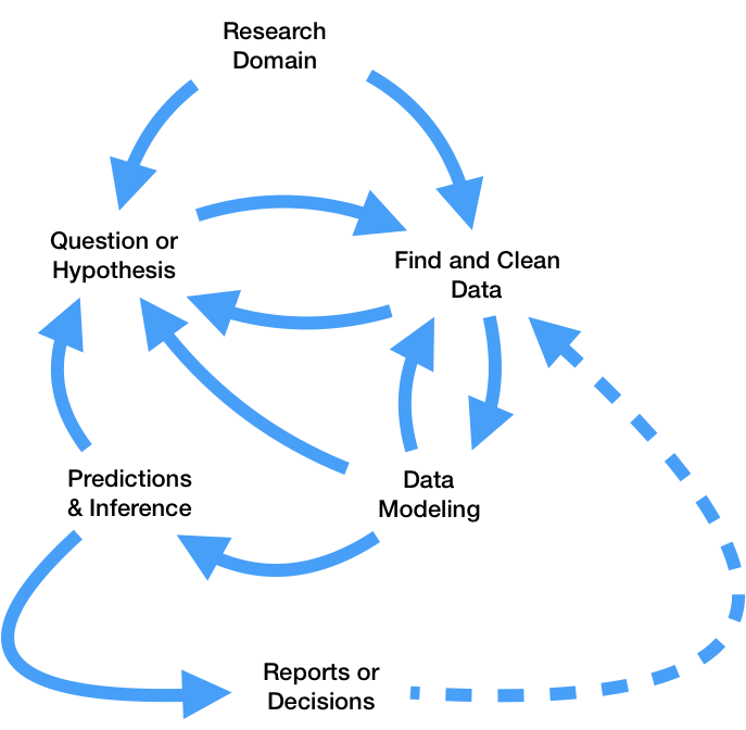
Lecture 20 – Modeling and Linear Regression

DSC 80, Spring 2023

Agenda

  • Modeling.
  • Case study: Restaurant tips 🧑‍🍳.
  • Regression in sklearn.

Modeling

Reflection

So far this quarter, we've learned how to:

  • Extract information from tabular data using pandas and regular expressions.
  • Clean data so that it best represents a data generating process.
    • Missingness analyses and imputation.
  • Collect data from the internet through scraping and APIs, and parse it using BeautifulSoup.
  • Perform exploratory data analysis through aggregation, visualization, and the computation of summary statistics like TF-IDF.
  • Infer about the relationships between samples and populations through hypothesis and permutation testing.
  • We haven't learned how to make predictions.

Modeling

  • Data generating process: A real-world phenomena that we are interested in studying.
    • Example: Every year, city employees are hired and fired, earn salaries and benefits, etc.
    • Unless we work for the city, we can't observe this process directly.
  • Model: A theory about the data generating process.
    • Example: If an employee is $X$ years older than average, then they will make $100,000 in salary.
  • Fit Model: A model that is learned from a particular set of observations, i.e. training data.
    • Example: If an employee is 5 years older than average, they will make $100,000 in salary.
    • How is this estimate determined? What makes it "good"?

Goals of modeling

  1. To make accurate predictions regarding unseen data drawn from the data generating process.
    • Given this dataset of past UCSD data science students' salaries, can we predict your future salary? (regression)
    • Given this dataset of images, can we predict if this new image is of a dog, cat, or zebra? (classification)
  1. To make inferences about the structure of the data generating process, i.e. to understand complex phenomena.
    • Is there a linear relationship between the heights of children and the heights of their biological mothers?
    • The weights of smoking and non-smoking mothers' babies babies in my sample are different – how confident am I that this difference exists in the population?
  • Of the two focuses of models, we will focus on prediction.
  • In the above taxonomy, we will focus on supervised learning.

Features

  • A feature is a measurable property of a phenomenon being observed.
    • Other terms for "feature" include "(explanatory) variable" and "attribute".
    • Typically, features are the inputs to models.
  • In DataFrames, features typically correspond to columns, while rows typically correspond to different individuals.
  • There are two types of features:
    • Features that come as part of a dataset, e.g. weight and height.
    • Features that we create, e.g. $\text{BMI} = \frac{\text{weight (kg)}}{\text{[height (m)]}^2}$.
  • Example: TF-IDF is a feature we've created that summarizes documents!

Example: Restaurant tips 🧑‍🍳

About the data

What features does the dataset contain?

In [2]:
# The dataset is built into plotly (and seaborn)!
tips = px.data.tips()
tips
Out[2]:
total_bill tip sex smoker day time size
0 16.99 1.01 Female No Sun Dinner 2
1 10.34 1.66 Male No Sun Dinner 3
2 21.01 3.50 Male No Sun Dinner 3
3 23.68 3.31 Male No Sun Dinner 2
4 24.59 3.61 Female No Sun Dinner 4
... ... ... ... ... ... ... ...
239 29.03 5.92 Male No Sat Dinner 3
240 27.18 2.00 Female Yes Sat Dinner 2
241 22.67 2.00 Male Yes Sat Dinner 2
242 17.82 1.75 Male No Sat Dinner 2
243 18.78 3.00 Female No Thur Dinner 2

244 rows × 7 columns

Predicting tips

  • Goal: Given various information about a table at a restaurant, we want to predict the tip that a server will earn.
  • Why might a server be interested in doing this?
    • To determine which tables are likely to tip the most (inference).
    • To predict earnings over the next month (prediction).

Exploratory data analysis (EDA)

  • The most natural feature to look at first is 'total_bill'.
  • As such, we should explore the relationship between 'total_bill' and 'tip', as well as the distributions of both columns individually.
  • As we do so, try to describe each distribution in words.

Visualizing distributions

In [3]:
tips.plot(kind='scatter', 
          x='total_bill', y='tip',
          title='Tip vs. Total Bill',
          template=TEMPLATE)
In [4]:
tips.plot(kind='hist', 
          x='total_bill', 
          title='Distribution of Total Bill',
          nbins=50,
          template=TEMPLATE)
In [5]:
tips.plot(kind='hist', 
          x='tip', 
          title='Distribution of Tip',
          nbins=50,
          template=TEMPLATE)

Observations

'total_bill' 'tip'
Right skewed Right skewed
Mean around $20 Mean around $3
Mode around $16 Possibly bimodal at \$2 and \$3?
No particularly large bills Large outliers?

Model #1: Constant

  • Let's start simple, by ignoring all features. Suppose our model assumes every tip is given by a constant dollar amount:
$$\text{tip} = h^{\text{true}}$$
  • Model: There is a single tip amount $h^{\text{true}}$ that all customers pay.
    • Correct? No!
    • Useful? Perhaps. An estimate of $h^{\text{true}}$, denoted by $h^*$, can allow us to predict future tips.
  • The true parameter $h^{\text{true}}$ is determined by the universe (i.e. the data generating process).
    • We can't observe the true parameter; we need to estimate it from the data.
    • Hence, our estimate depends on our dataset!
George Box
"All models are wrong, but some are useful."

"Since all models are wrong the scientist cannot obtain a "correct" one by excessive elaboration. On the contrary following William of Occam he should seek an economical description of natural phenomena. Just as the ability to devise simple but evocative models is the signature of the great scientist so overelaboration and overparameterization is often the mark of mediocrity."

"Since all models are wrong the scientist must be alert to what is importantly wrong. It is inappropriate to be concerned about mice when there are tigers abroad."

Estimating $h^{\text{true}}$

  • There are several ways we could estimate $h^{\text{true}}$.
    • We could use domain knowledge (e.g. everyone clicks the $1 tip option when buying coffee).
  • From DSC 40A, we already know one way:
    • Choose a loss function, which measures how "good" a single prediction is.
    • Minimize empirical risk, to find the best estimate for the dataset that we have.

Empirical risk minimization

  • Depending on which loss function we choose, we will end up with different $h^*$ (which are estimates of $h^{\text{true}})$.
  • If we choose squared loss, then our empirical risk is mean squared error:
$$\text{MSE} = \frac{1}{n} \sum_{i = 1}^n ( y_i - h )^2 \overset{\text{calculus}}\implies h^* = \text{mean}(y)$$
  • If we choose absolute loss, then our empirical risk is mean absolute error:
$$\text{MAE} = \frac{1}{n} \sum_{i = 1}^n | y_i - h | \overset{\text{algebra}}\implies h^* = \text{median}(y)$$

The mean tip

Let's suppose we choose squared loss, meaning that $h^* = \text{mean}(y)$.

In [6]:
mean_tip = tips['tip'].mean()
mean_tip
Out[6]:
2.99827868852459

Let's visualize this prediction.

In [7]:
# Unfortunately, the code to visualize a scatter plot and a line
# in plotly is not all that concise.
fig = go.Figure()

fig.add_trace(go.Scatter(
    x=tips['total_bill'], 
    y=tips['tip'], 
    mode='markers',
    name='Original Data')
)

fig.add_trace(go.Scatter(
    x=[0, 60],
    y=[mean_tip, mean_tip],
    mode='lines',
    name='Constant Prediction (Mean)'
))

fig.update_layout(showlegend=True, title='Tip vs. Total Bill',
                  xaxis_title='Total Bill', yaxis_title='Tip',
                  template=TEMPLATE)
fig.update_xaxes(range=[0, 60])

Note that to make predictions, this model ignores total bill (and all other features), and predicts the same tip for all tables.

The quality of predictions

  • Question: How can we quantify how good this constant prediction is at predicting tips in our training data – that is, the data we used to fit the model?
  • One answer: use the mean squared error. If $y_i$ represents the $i$th actual value and $H(x_i)$ represents the $i$th predicted value, then:
$$\text{MSE} = \frac{1}{n} \sum_{i = 1}^n \big( y_i - H(x_i) \big)^2$$
In [8]:
np.mean((tips['tip'] - mean_tip) ** 2)
Out[8]:
1.9066085124966412
In [9]:
# The same! A fact from 40A.
np.var(tips['tip'])
Out[9]:
1.9066085124966412
  • Issue: The units of MSE are "dollars squared", which are a little hard to interpret.

Root mean squared error

  • Often, to measure the quality of a regression model's predictions, we will use the root mean squared error (RMSE):
$$\text{RMSE} = \sqrt{\frac{1}{n} \sum_{i = 1}^n \big( y_i - H(x_i) \big)^2}$$
  • The units of the RMSE are the same as the units of the original $y$ values – dollars, in this case.
  • Important: Minimizing MSE is the same as minimizing RMSE; the constant tip $h^*$ that minimizes MSE is the same $h^*$ that minimizes RMSE.

Computing and storing the RMSE

Since we'll compute the RMSE for our future models too, we'll define a function that can compute it for us.

In [10]:
def rmse(actual, pred):
    return np.sqrt(np.mean((actual - pred) ** 2))

Let's compute the RMSE of our constant tip's predictions, and store it in a dictionary that we can refer to later on.

In [11]:
rmse(tips['tip'], mean_tip)
Out[11]:
1.3807999538298954
In [12]:
rmse_dict = {}
rmse_dict['constant tip amount'] = rmse(tips['tip'], mean_tip)
rmse_dict
Out[12]:
{'constant tip amount': 1.3807999538298954}

Key idea: Since the mean minimizes RMSE for the constant model, it is impossible to change the mean_tip argument above to another number and yield a lower RMSE.

Model #2: Simple linear regression using total bill

  • We haven't yet used any of the features in the dataset. The first natural feature to look at is 'total_bill'.
In [13]:
tips.head()
Out[13]:
total_bill tip sex smoker day time size
0 16.99 1.01 Female No Sun Dinner 2
1 10.34 1.66 Male No Sun Dinner 3
2 21.01 3.50 Male No Sun Dinner 3
3 23.68 3.31 Male No Sun Dinner 2
4 24.59 3.61 Female No Sun Dinner 4
  • We can fit a simple linear model to predict tips as a function of total bill:
$$\text{predicted tip} = w_0 + w_1 \cdot \text{total bill}$$
  • This is a reasonable thing to do, because total bills and tips appeared to be linearly associated when we visualized them on a scatter plot a few slides ago.

Recap: Simple linear regression

A simple linear regression model is a linear model with a single feature, as we have here. For any total bill $x_i$, the predicted tip $H(x_i)$ is given by

$$H(x_i) = w_0 + w_1x_i$$
  • Question: How do we determine which intercept, $w_0$, and slope, $w_1$, to use?
  • One answer: Pick the $w_0$ and $w_1$ that minimize mean squared error. If $x_i$ and $y_i$ correspond to the $i$th total bill and tip, respectively, then:
$$\begin{align*}\text{MSE} &= \frac{1}{n} \sum_{i = 1}^n \big( y_i - H(x_i) \big)^2 \\ &= \frac{1}{n} \sum_{i = 1}^n \big( y_i - w_0 - w_1x_i \big)^2\end{align*}$$
  • Key idea: The lower the MSE on our training data is, the "better" the model fits the training data.

Empirical risk minimization, by hand

$$\begin{align*}\text{MSE} &= \frac{1}{n} \sum_{i = 1}^n \big( y_i - w_0 - w_1x_i \big)^2\end{align*}$$
  • In DSC 40A, you found the formulas for the best intercept, $w_0^*$, and the best slope, $w_1^*$, through calculus.
    • The resulting line, $H(x_i) = w_0^* + w_1^* x_i$, is called the line of best fit, or the regression line.
  • Specifically, if $r$ is the correlation coefficient, $\sigma_x$ and $\sigma_y$ are the standard deviations of $x$ and $y$, and $\bar{x}$ and $\bar{y}$ are the means of $x$ and $y$, then:
$$w_1^* = r \cdot \frac{\sigma_y}{\sigma_x}$$$$w_0^* = \bar{y} - w_1^* \bar{x}$$

Regression in sklearn

sklearn

  • sklearn (scikit-learn) implements many common steps in the feature and model creation pipeline.
    • It is widely used throughout industry and academia.
  • It interfaces with numpy arrays, and to an extent, pandas DataFrames.
  • Huge benefit: the documentation online is excellent.

The LinearRegression class

  • sklearn comes with several subpackages, including linear_model and tree, each of which contains several classes of models.
  • We'll start with the LinearRegression class from linear_model.
In [14]:
from sklearn.linear_model import LinearRegression
  • Important: From the documentation, we have:

LinearRegression fits a linear model with coefficients w = (w1, …, wp) to minimize the residual sum of squares between the observed targets in the dataset, and the targets predicted by the linear approximation.

  • In other words, LinearRegression minimizes mean squared error by default! (Per the documentation, it also includes an intercept term by default.)
In [15]:
LinearRegression?

Fitting a simple linear model

First, we must instantiate a LinearRegression object and fit it. By calling fit, we are saying "minimize mean squared error on this dataset and find $w^*$."

In [16]:
model = LinearRegression()

# Note that there are two arguments to fit – X and y!
# (It is not necessary to write X= and y=)
model.fit(X=tips[['total_bill']], y=tips['tip'])
Out[16]:
LinearRegression()

After fitting, we can access $w^*$ – that is, the best slope and intercept.

In [17]:
model.intercept_, model.coef_
Out[17]:
(0.9202696135546731, array([0.10502452]))

These coefficients tell us that the "best way" (according to squared loss) to make tip predictions using a linear model is using:

$$\text{predicted tip} = 0.92 + 0.105 \cdot \text{total bill}$$

This model assumes people tip by:

  • Tipping a constant 92 cents.
  • Tipping 10.5% for every dollar spent.

Let's visualize this model, along with our previous model.

In [18]:
fig.add_trace(go.Scatter(
    x=[0, 60],
    y=model.predict([[0], [60]]),
    mode='lines',
    name='Linear: Total Bill Only'
))
/Users/larry/opt/anaconda3/envs/dsc80/lib/python3.8/site-packages/sklearn/base.py:441: UserWarning:

X does not have valid feature names, but LinearRegression was fitted with feature names

Visually, our linear model seems to be a better fit for our dataset than our constant model.

  • Can we quantify whether or not it is better?
  • Does it better reflect reality?

Making predictions

Fit LinearRegression objects also have a predict method, which can be used to predict tips for any total bill, new or old.

In [19]:
model.predict([[15]])
/Users/larry/opt/anaconda3/envs/dsc80/lib/python3.8/site-packages/sklearn/base.py:441: UserWarning:

X does not have valid feature names, but LinearRegression was fitted with feature names

Out[19]:
array([2.49563737])
In [20]:
# The input to model.predict **must** be a 2D list/array.
model.predict([[15],
               [4],
               [100]])
/Users/larry/opt/anaconda3/envs/dsc80/lib/python3.8/site-packages/sklearn/base.py:441: UserWarning:

X does not have valid feature names, but LinearRegression was fitted with feature names

Out[20]:
array([ 2.49563737,  1.34036768, 11.42272135])
In [21]:
model.predict(np.array(
    [15, 4, 100]
).reshape(-1, 1))
/Users/larry/opt/anaconda3/envs/dsc80/lib/python3.8/site-packages/sklearn/base.py:441: UserWarning:

X does not have valid feature names, but LinearRegression was fitted with feature names

Out[21]:
array([ 2.49563737,  1.34036768, 11.42272135])

Comparing models

If we want to compute the RMSE of our model on the training data, we need to find its predictions on every row in the training data, tips.

In [22]:
all_preds = model.predict(tips[['total_bill']])
In [23]:
rmse_dict['one feature: total bill'] = rmse(tips['tip'], all_preds)
rmse_dict
Out[23]:
{'constant tip amount': 1.3807999538298954,
 'one feature: total bill': 1.0178504025697377}
  • The RMSE of our simple linear model is lower than that of our constant model, which means it does a better job at modeling the training data than our constant model.
  • It is impossible for the RMSE on the training data to increase as we add more features to the same model. However, the RMSE may increase on unseen data by adding more features; we'll discuss this idea more soon.

Model #3: Multiple linear regression using total bill and table size

  • There are still many features in tips we haven't touched:
In [24]:
tips.head()
Out[24]:
total_bill tip sex smoker day time size
0 16.99 1.01 Female No Sun Dinner 2
1 10.34 1.66 Male No Sun Dinner 3
2 21.01 3.50 Male No Sun Dinner 3
3 23.68 3.31 Male No Sun Dinner 2
4 24.59 3.61 Female No Sun Dinner 4
  • Let's try using another feature – table size. Such a model would predict tips using:
$$\text{predicted tip} = w_0 + w_1 \cdot \text{total bill} + w_2 \cdot \text{table size}$$

Multiple linear regression

To find the optimal parameters $w^*$, we will again use sklearn's LinearRegression class. The code is not all that different!

In [25]:
model_two = LinearRegression()
model_two.fit(X=tips[['total_bill', 'size']], y=tips['tip'])
Out[25]:
LinearRegression()
In [26]:
model_two.intercept_, model_two.coef_
Out[26]:
(0.6689447408125031, array([0.09271334, 0.19259779]))
In [27]:
model_two.predict([[25, 4]])
/Users/larry/opt/anaconda3/envs/dsc80/lib/python3.8/site-packages/sklearn/base.py:441: UserWarning:

X does not have valid feature names, but LinearRegression was fitted with feature names

Out[27]:
array([3.75716934])

What does this model look like?

Plane of best fit ✈️

Here, we must draw a 3D scatter plot and plane, with one axis for total bill, one axis for table size, and one axis for tip. The code below does this.

In [28]:
XX, YY = np.mgrid[0:50:2, 0:8:1]
Z = model_two.intercept_ + model_two.coef_[0] * XX + model_two.coef_[1] * YY
plane = go.Surface(x=XX, y=YY, z=Z, colorscale='Oranges')

fig = go.Figure(data=[plane])
fig.add_trace(go.Scatter3d(x=tips['total_bill'], 
                           y=tips['size'], 
                           z=tips['tip'], mode='markers', marker = {'color': '#656DF1'}))

fig.update_layout(scene = dict(
    xaxis_title='total bill',
    yaxis_title='table size',
    zaxis_title='tip'),
  title='Tip vs. Total Bill and Table Size',
    width=1000, height=800)

Comparing models, again

How does our two-feature linear model stack up to our single feature linear model and our constant model?

In [29]:
rmse_dict['two features'] = rmse(
    tips['tip'], model_two.predict(tips[['total_bill', 'size']])
)
In [30]:
rmse_dict
Out[30]:
{'constant tip amount': 1.3807999538298954,
 'one feature: total bill': 1.0178504025697377,
 'two features': 1.007256127114662}
  • The RMSE of our two-feature model is the lowest of the three models we've looked at so far, but not by much. We didn't gain much by adding table size to our linear model.
  • It's also not clear whether table sizes are practically useful in predicting tips.

Conclusion

  • We built three models:
    • A constant model: $\text{predicted tip} = h^*$.
    • A simple linear regression model: $\text{predicted tip} = w_0^* + w_1^* \cdot \text{total bill}$.
    • A multiple linear regression model: $\text{predicted tip} = w_0^* + w_1^* \cdot \text{total bill} + w_2^* \cdot \text{table size}$.
  • As we added more features, our RMSEs decreased.
    • This was guaranteed to happen, since we were only looking at our training data.
  • It is not clear that the final linear model is actually "better"; it doesn't seem to reflect reality better than the previous models.

Summary, next time

Summary

  • A model is an assumption about a data generating process.
    • Models can be used for both inference and prediction.
    • All models are wrong (because they are oversimplifications of reality), but even simple models can be useful in practice.
  • A feature is a measurable property of a phenomenon being observed, typically used as input to a model.
  • The LinearRegression class in sklearn.linear_model provides an implementation of least squares linear regression that works with multiple features.

Next time

  • How do we encode categorical features?
    • What if they're nominal?
    • What if they're ordinal?
  • How do we create good features?
  • How else can we compare linear models?