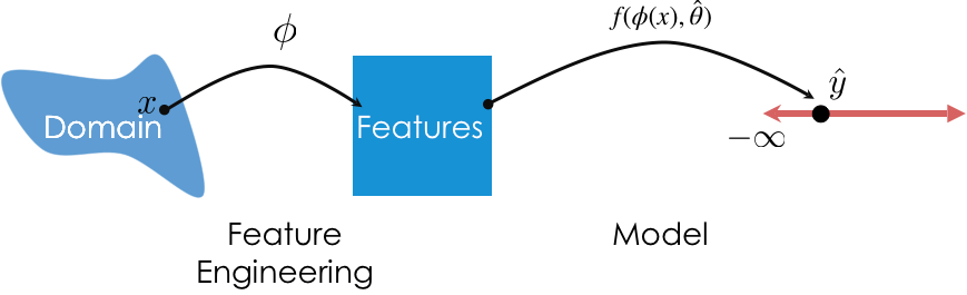
The modeling process
import pandas as pd
import numpy as np
import os

import plotly.express as px
import plotly.graph_objects as go
pd.options.plotting.backend = 'plotly'
TEMPLATE = 'seaborn'

from sklearn.linear_model import LinearRegression

import util
sklearn.We can perform all of the above directly in sklearn!
preprocessing and linear_models¶For the feature engineering step of the modeling pipeline, we will use sklearn's preprocessing module.

For the model creation step of the modeling pipeline, we will use sklearn's linear_model module, as we've already seen. linear_model.LinearRegression is an example of an estimator class.

sklearn¶numpy array.sklearn only looks at the values (i.e. it calls to_numpy() on input DataFrames).numpy array (never a DataFrame or Series).sklearn, are classes, not functions, meaning you need to instantiate them and call their methods.We'll continue working with our trusty tips dataset.
tips = px.data.tips()
tips.head()
| total_bill | tip | sex | smoker | day | time | size | |
|---|---|---|---|---|---|---|---|
| 0 | 16.99 | 1.01 | Female | No | Sun | Dinner | 2 |
| 1 | 10.34 | 1.66 | Male | No | Sun | Dinner | 3 |
| 2 | 21.01 | 3.50 | Male | No | Sun | Dinner | 3 |
| 3 | 23.68 | 3.31 | Male | No | Sun | Dinner | 2 |
| 4 | 24.59 | 3.61 | Female | No | Sun | Dinner | 4 |
Binarizer¶The Binarizer transformer allows us to map a quantitative sequence to a sequence of 1s and 0s, depending on whether values are above or below a threshold.
| Property | Example | Description |
|---|---|---|
| Initialize with parameters | binar = Binarizer(thresh) |
set x=1 if x > thresh, else 0 |
| Transform data in a dataset | feat = binar.transform(data) |
Binarize all columns in data |
First, we need to import the relevant class from sklearn.preprocessing. (Tip: import just the relevant classes you need from sklearn.)
from sklearn.preprocessing import Binarizer
Let's try binarizing 'total_bill'. We'll say a "large" bill is one that is strictly greater than $20.
tips['total_bill'].head()
0    16.99
1    10.34
2    21.01
3    23.68
4    24.59
Name: total_bill, dtype: float64
First, we initialize a Binarizer object with the threshold we want.
bi = Binarizer(threshold=20)
Then, we call bi's transform method and pass it the data we'd like to transform. Note that its input and output are both 2D.
transformed_bills = bi.transform(tips[['total_bill']]) # Must give transform a 2D array/DataFrame.
transformed_bills[:5]
/Users/larry/opt/anaconda3/envs/dsc80/lib/python3.8/site-packages/sklearn/base.py:434: UserWarning: X has feature names, but Binarizer was fitted without feature names
  warnings.warn(
array([[0.],
       [0.],
       [1.],
       [1.],
       [1.]])
StdScaler¶StdScaler standardizes data using the mean and standard deviation of the data.Binarizer, StdScaler requires some knowledge (mean and SD) of the dataset before transforming.fit an StdScaler transformer before we can use the transform method.StdScaler¶It only makes sense to standardize the already-quantitative features of tips, so let's select just those.
tips_quant = tips[['total_bill', 'size']]
tips_quant.head()
| total_bill | size | |
|---|---|---|
| 0 | 16.99 | 2 |
| 1 | 10.34 | 3 |
| 2 | 21.01 | 3 |
| 3 | 23.68 | 2 |
| 4 | 24.59 | 4 |
Let's initialize a StandardScaler object.
from sklearn.preprocessing import StandardScaler
stdscaler = StandardScaler()
Note that the following does not work! The error message is very helpful.
stdscaler.transform(tips_quant)
---------------------------------------------------------------------------
NotFittedError                            Traceback (most recent call last)
Input In [10], in <cell line: 1>()
----> 1 stdscaler.transform(tips_quant)

File ~/opt/anaconda3/envs/dsc80/lib/python3.8/site-packages/sklearn/preprocessing/_data.py:970, in StandardScaler.transform(self, X, copy)
    955 def transform(self, X, copy=None):
    956     """Perform standardization by centering and scaling.
    957
    958     Parameters
   (...)
    968         Transformed array.
    969     """
--> 970     check_is_fitted(self)
    972     copy = copy if copy is not None else self.copy
    973     X = self._validate_data(
    974         X,
    975         reset=False,
   (...)
    980         force_all_finite="allow-nan",
    981     )

File ~/opt/anaconda3/envs/dsc80/lib/python3.8/site-packages/sklearn/utils/validation.py:1208, in check_is_fitted(estimator, attributes, msg, all_or_any)
   1203     fitted = [
   1204         v for v in vars(estimator) if v.endswith("_") and not v.startswith("__")
   1205     ]
   1207 if not fitted:
-> 1208     raise NotFittedError(msg % {"name": type(estimator).__name__})

NotFittedError: This StandardScaler instance is not fitted yet. Call 'fit' with appropriate arguments before using this estimator.
Instead, we need to first call the fit method on stdscaler.
# This is like saying "determine the mean and SD of each column in tips_quant".
stdscaler.fit(tips_quant)
StandardScaler()
Now, transform will work.
# First column is 'total_bill', second column is 'size'.
tips_quant_z = stdscaler.transform(tips_quant)
tips_quant_z[:5]
array([[-0.31471131, -0.60019263],
       [-1.06323531,  0.45338292],
       [ 0.1377799 ,  0.45338292],
       [ 0.4383151 , -0.60019263],
       [ 0.5407447 ,  1.50695847]])
We can also access the mean and variance stdscaler computed for each column:
stdscaler.mean_
array([19.78594262, 2.56967213])
stdscaler.var_
array([78.92813149, 0.9008835 ])
Note that we can call transform on DataFrames other than tips_quant. We will do this often – fit a transformer on one dataset (training data) and use it to transform other datasets (test data).
stdscaler.transform(tips_quant.sample(5))
array([[-1.02834171, -0.60019263],
       [ 0.0792487 , -0.60019263],
       [ 0.66681191,  0.45338292],
       [ 0.97410071, -0.60019263],
       [ 0.1377799 ,  0.45338292]])
StdScaler summary¶| Property | Example | Description |
|---|---|---|
| Initialize with parameters | stdscaler = StandardScaler() |
z-score the data (no parameters) |
| Fit the transformer | stdscaler.fit(X) |
Compute the mean and SD of X |
| Transform data in a dataset | feat = stdscaler.transform(X_new) |
z-score X_new with mean and SD of X |
OneHotEncoder¶Let's keep just the categorical columns in tips.
tips_cat = tips[['sex', 'smoker', 'day', 'time']]
tips_cat.head()
| sex | smoker | day | time | |
|---|---|---|---|---|
| 0 | Female | No | Sun | Dinner |
| 1 | Male | No | Sun | Dinner |
| 2 | Male | No | Sun | Dinner |
| 3 | Male | No | Sun | Dinner |
| 4 | Female | No | Sun | Dinner |
Like StdScaler, we will need to fit our OneHotEncoder transformer before it can transform anything.
from sklearn.preprocessing import OneHotEncoder
ohe = OneHotEncoder()
ohe.fit(tips_cat)
OneHotEncoder()
We can look at the unique values (i.e. categories) in each column by using the categories_ attribute:
ohe.categories_
[array(['Female', 'Male'], dtype=object),
 array(['No', 'Yes'], dtype=object),
 array(['Fri', 'Sat', 'Sun', 'Thur'], dtype=object),
 array(['Dinner', 'Lunch'], dtype=object)]
ohe.transform(tips_cat)
<244x10 sparse matrix of type '<class 'numpy.float64'>'
	with 976 stored elements in Compressed Sparse Row format>
Since the resulting matrix is sparse – most of its elements are 0 – sklearn uses a more efficient representation than a regular numpy array. That's no issue, though:
ohe.transform(tips_cat).toarray()
array([[1., 0., 1., ..., 0., 1., 0.],
       [0., 1., 1., ..., 0., 1., 0.],
       [0., 1., 1., ..., 0., 1., 0.],
       ...,
       [0., 1., 0., ..., 0., 1., 0.],
       [0., 1., 1., ..., 0., 1., 0.],
       [1., 0., 1., ..., 1., 1., 0.]])
Notice that the column names from tips_cat are no longer stored anywhere (remember, fit converts the input to a numpy array before proceeding).
We can use the get_feature_names method on ohe to access the names of the one-hot-encoded columns, though:
ohe.get_feature_names() # x0, x1, x2, and x3 correspond to column names in tips_cat.
/Users/larry/opt/anaconda3/envs/dsc80/lib/python3.8/site-packages/sklearn/utils/deprecation.py:87: FutureWarning: Function get_feature_names is deprecated; get_feature_names is deprecated in 1.0 and will be removed in 1.2. Please use get_feature_names_out instead.
  warnings.warn(msg, category=FutureWarning)
array(['x0_Female', 'x0_Male', 'x1_No', 'x1_Yes', 'x2_Fri', 'x2_Sat',
       'x2_Sun', 'x2_Thur', 'x3_Dinner', 'x3_Lunch'], dtype=object)
pd.DataFrame(ohe.transform(tips_cat).toarray(),
             columns=ohe.get_feature_names()) # If we need a DataFrame back, for some reason.
/Users/larry/opt/anaconda3/envs/dsc80/lib/python3.8/site-packages/sklearn/utils/deprecation.py:87: FutureWarning: Function get_feature_names is deprecated; get_feature_names is deprecated in 1.0 and will be removed in 1.2. Please use get_feature_names_out instead.
  warnings.warn(msg, category=FutureWarning)
| x0_Female | x0_Male | x1_No | x1_Yes | x2_Fri | x2_Sat | x2_Sun | x2_Thur | x3_Dinner | x3_Lunch | |
|---|---|---|---|---|---|---|---|---|---|---|
| 0 | 1.0 | 0.0 | 1.0 | 0.0 | 0.0 | 0.0 | 1.0 | 0.0 | 1.0 | 0.0 |
| 1 | 0.0 | 1.0 | 1.0 | 0.0 | 0.0 | 0.0 | 1.0 | 0.0 | 1.0 | 0.0 |
| 2 | 0.0 | 1.0 | 1.0 | 0.0 | 0.0 | 0.0 | 1.0 | 0.0 | 1.0 | 0.0 |
| 3 | 0.0 | 1.0 | 1.0 | 0.0 | 0.0 | 0.0 | 1.0 | 0.0 | 1.0 | 0.0 |
| 4 | 1.0 | 0.0 | 1.0 | 0.0 | 0.0 | 0.0 | 1.0 | 0.0 | 1.0 | 0.0 |
| ... | ... | ... | ... | ... | ... | ... | ... | ... | ... | ... |
| 239 | 0.0 | 1.0 | 1.0 | 0.0 | 0.0 | 1.0 | 0.0 | 0.0 | 1.0 | 0.0 |
| 240 | 1.0 | 0.0 | 0.0 | 1.0 | 0.0 | 1.0 | 0.0 | 0.0 | 1.0 | 0.0 |
| 241 | 0.0 | 1.0 | 0.0 | 1.0 | 0.0 | 1.0 | 0.0 | 0.0 | 1.0 | 0.0 |
| 242 | 0.0 | 1.0 | 1.0 | 0.0 | 0.0 | 1.0 | 0.0 | 0.0 | 1.0 | 0.0 |
| 243 | 1.0 | 0.0 | 1.0 | 0.0 | 0.0 | 0.0 | 0.0 | 1.0 | 1.0 | 0.0 |
244 rows × 10 columns
So far, we've used transformers for feature engineering and models for prediction. We can combine these steps into a single Pipeline.
Pipelines in sklearn¶Pipeline, we must provide a list with zero or more transformers followed by a single model.fit methods, and all but the last must have transform methods.pl = Pipeline([feat_trans1, feat_trans2, ..., mdl]).
Pipeline is instantiated, you can fit all steps (transformers and model) using a single call to the fit method.pl.fit(X, y)
pl.predict.Pipeline with must be a list of tuples, wherePipeline¶Let's build a Pipeline that:
tips.tips_cat = tips[['sex', 'smoker', 'day', 'time']]
tips_cat.head()
| sex | smoker | day | time | |
|---|---|---|---|---|
| 0 | Female | No | Sun | Dinner |
| 1 | Male | No | Sun | Dinner |
| 2 | Male | No | Sun | Dinner |
| 3 | Male | No | Sun | Dinner |
| 4 | Female | No | Sun | Dinner |
from sklearn.pipeline import Pipeline
pl = Pipeline([
    ('one-hot', OneHotEncoder()),
    ('lin-reg', LinearRegression())
])
Now that pl is instantiated, we fit it the same way we would fit the individual steps.
pl.fit(tips_cat, tips['tip'])
Pipeline(steps=[('one-hot', OneHotEncoder()), ('lin-reg', LinearRegression())])
Now, to make predictions using raw data, all we need to do is use pl.predict:
pl.predict([['Female', 'Yes', 'Sat', 'Lunch']])
/Users/larry/opt/anaconda3/envs/dsc80/lib/python3.8/site-packages/sklearn/base.py:441: UserWarning: X does not have valid feature names, but OneHotEncoder was fitted with feature names
  warnings.warn(
array([2.41792163])
pl.predict(tips_cat.iloc[:5])
array([3.10415414, 3.27436302, 3.27436302, 3.27436302, 3.10415414])
pl performs both feature transformation and prediction with just a single call to predict!
We can access individual "steps" of a Pipeline through the named_steps attribute:
pl.named_steps
{'one-hot': OneHotEncoder(), 'lin-reg': LinearRegression()}
pl.named_steps['one-hot'].transform(tips_cat).toarray()
array([[1., 0., 1., ..., 0., 1., 0.],
       [0., 1., 1., ..., 0., 1., 0.],
       [0., 1., 1., ..., 0., 1., 0.],
       ...,
       [0., 1., 0., ..., 0., 1., 0.],
       [0., 1., 1., ..., 0., 1., 0.],
       [1., 0., 1., ..., 1., 1., 0.]])
pl.named_steps['lin-reg'].coef_
array([-0.08510444,  0.08510444, -0.04216238,  0.04216238, -0.20256076,
       -0.12962763,  0.13756057,  0.19462781,  0.25168453, -0.25168453])
pl also has a score method, the same way a fit LinearRegression instance does:
pl.score(tips_cat, tips['tip'])
0.027496790201475663
Pipelines¶ColumnTransformer.ColumnTransformer using a list of tuples, where:OneHotEncoder()).ColumnTransformer is extremely useful, but it was only added to sklearn in 2018!ColumnTransformer¶from sklearn.compose import ColumnTransformer
Let's perform different transformations on the quantitative and categorical features of tips (note that we are not transforming 'tip').
tips_features = tips.drop('tip', axis=1)
tips_features.head()
| total_bill | sex | smoker | day | time | size | |
|---|---|---|---|---|---|---|
| 0 | 16.99 | Female | No | Sun | Dinner | 2 |
| 1 | 10.34 | Male | No | Sun | Dinner | 3 |
| 2 | 21.01 | Male | No | Sun | Dinner | 3 |
| 3 | 23.68 | Male | No | Sun | Dinner | 2 |
| 4 | 24.59 | Female | No | Sun | Dinner | 4 |
'total_bill' column untouched.'size' column, we will apply the Binarizer transformer with a threshold of 2 (big tables vs. small tables).OneHotEncoder transformer.| size | x0_Female | x0_Male | x1_No | x1_Yes | x2_Fri | x2_Sat | x2_Sun | x2_Thur | x3_Dinner | x3_Lunch | total_bill | |
|---|---|---|---|---|---|---|---|---|---|---|---|---|
| 0 | 0 | 1.0 | 0.0 | 1.0 | 0.0 | 0.0 | 0.0 | 1.0 | 0.0 | 1.0 | 0.0 | 16.99 |
| 1 | 1 | 0.0 | 1.0 | 1.0 | 0.0 | 0.0 | 0.0 | 1.0 | 0.0 | 1.0 | 0.0 | 10.34 |
| 2 | 1 | 0.0 | 1.0 | 1.0 | 0.0 | 0.0 | 0.0 | 1.0 | 0.0 | 1.0 | 0.0 | 21.01 |
| 3 | 0 | 0.0 | 1.0 | 1.0 | 0.0 | 0.0 | 0.0 | 1.0 | 0.0 | 1.0 | 0.0 | 23.68 |
| 4 | 1 | 1.0 | 0.0 | 1.0 | 0.0 | 0.0 | 0.0 | 1.0 | 0.0 | 1.0 | 0.0 | 24.59 |
Pipeline using a ColumnTransformer¶Let's start by creating our ColumnTransformer.
preproc = ColumnTransformer(
    transformers=[
        ('size', Binarizer(threshold=2), ['size']),
        ('categorical_cols', OneHotEncoder(), ['sex', 'smoker', 'day', 'time'])
    ],
    remainder='passthrough' # Specify what to do with all other columns ('total_bill' here) – drop or passthrough.
)
Now, let's create a Pipeline using preproc as a transformer, and fit it:
pl = Pipeline([
    ('preprocessor', preproc),
    ('lin-reg', LinearRegression())
])
pl.fit(tips_features, tips['tip'])
Pipeline(steps=[('preprocessor',
                 ColumnTransformer(remainder='passthrough',
                                   transformers=[('size',
                                                  Binarizer(threshold=2),
                                                  ['size']),
                                                 ('categorical_cols',
                                                  OneHotEncoder(),
                                                  ['sex', 'smoker', 'day',
                                                   'time'])])),
                ('lin-reg', LinearRegression())])
Prediction is as easy as calling predict:
tips_features.head()
| total_bill | sex | smoker | day | time | size | |
|---|---|---|---|---|---|---|
| 0 | 16.99 | Female | No | Sun | Dinner | 2 |
| 1 | 10.34 | Male | No | Sun | Dinner | 3 |
| 2 | 21.01 | Male | No | Sun | Dinner | 3 |
| 3 | 23.68 | Male | No | Sun | Dinner | 2 |
| 4 | 24.59 | Female | No | Sun | Dinner | 4 |
# Note that we fit the Pipeline using tips_features, not tips_features.head()!
pl.predict(tips_features.head())
array([2.73813307, 2.32343202, 3.3700388 , 3.36798392, 3.74755924])
We can even call each transformer in pl['preprocessor'] individually to re-create the transformed DataFrame. (There's no practical reason to do this, it's more for illustration.)
dfs = []
for trans in pl['preprocessor'].transformers_:
    if isinstance(trans[1], str) and trans[1] == 'passthrough':
        df = tips_features.iloc[:, trans[2]]
    else:
        vals = trans[1].transform(tips_features[trans[2]])
        columns = trans[2]
        if str(trans[1]) == 'OneHotEncoder()':
            vals = vals.toarray()
            columns = trans[1].get_feature_names()
        df = pd.DataFrame(vals, columns=columns)
    dfs.append(df)

pd.concat(dfs, axis=1)
/Users/larry/opt/anaconda3/envs/dsc80/lib/python3.8/site-packages/sklearn/utils/deprecation.py:87: FutureWarning: Function get_feature_names is deprecated; get_feature_names is deprecated in 1.0 and will be removed in 1.2. Please use get_feature_names_out instead.
  warnings.warn(msg, category=FutureWarning)
| size | x0_Female | x0_Male | x1_No | x1_Yes | x2_Fri | x2_Sat | x2_Sun | x2_Thur | x3_Dinner | x3_Lunch | total_bill | |
|---|---|---|---|---|---|---|---|---|---|---|---|---|
| 0 | 0 | 1.0 | 0.0 | 1.0 | 0.0 | 0.0 | 0.0 | 1.0 | 0.0 | 1.0 | 0.0 | 16.99 |
| 1 | 1 | 0.0 | 1.0 | 1.0 | 0.0 | 0.0 | 0.0 | 1.0 | 0.0 | 1.0 | 0.0 | 10.34 |
| 2 | 1 | 0.0 | 1.0 | 1.0 | 0.0 | 0.0 | 0.0 | 1.0 | 0.0 | 1.0 | 0.0 | 21.01 |
| 3 | 0 | 0.0 | 1.0 | 1.0 | 0.0 | 0.0 | 0.0 | 1.0 | 0.0 | 1.0 | 0.0 | 23.68 |
| 4 | 1 | 1.0 | 0.0 | 1.0 | 0.0 | 0.0 | 0.0 | 1.0 | 0.0 | 1.0 | 0.0 | 24.59 |
| ... | ... | ... | ... | ... | ... | ... | ... | ... | ... | ... | ... | ... |
| 239 | 1 | 0.0 | 1.0 | 1.0 | 0.0 | 0.0 | 1.0 | 0.0 | 0.0 | 1.0 | 0.0 | 29.03 |
| 240 | 0 | 1.0 | 0.0 | 0.0 | 1.0 | 0.0 | 1.0 | 0.0 | 0.0 | 1.0 | 0.0 | 27.18 |
| 241 | 0 | 0.0 | 1.0 | 0.0 | 1.0 | 0.0 | 1.0 | 0.0 | 0.0 | 1.0 | 0.0 | 22.67 |
| 242 | 0 | 0.0 | 1.0 | 1.0 | 0.0 | 0.0 | 1.0 | 0.0 | 0.0 | 1.0 | 0.0 | 17.82 |
| 243 | 0 | 1.0 | 0.0 | 1.0 | 0.0 | 0.0 | 0.0 | 0.0 | 1.0 | 1.0 | 0.0 | 18.78 |
244 rows × 12 columns
FunctionTransformer¶A transformer you'll often use as part of a ColumnTransformer is the FunctionTransformer, which enables you to use your own functions on entire columns. Think of it as the sklearn equivalent of apply.
from sklearn.preprocessing import FunctionTransformer
f = FunctionTransformer(np.sqrt)
f.transform([1, 2, 3])
array([1. , 1.41421356, 1.73205081])
Pipelines¶Pipelines are powerful because they allow you to perform feature engineering and training/prediction all through a single object.Pipeline does. Neural networks work similarly to sklearn Pipelines, in that they follow a well-defined sequence of steps to make predictions.Let's collect two samples $\{(x_i, y_i)\}$ from the same data generating process.
np.random.seed(23) # For reproducibility.

def sample_dgp(n=100):
    x = np.linspace(-2, 3, n)
    y = x ** 3 + (np.random.normal(0, 3, size=n))
    return pd.DataFrame({'x': x, 'y': y})

sample_1 = sample_dgp()
sample_2 = sample_dgp()
For now, let's just look at Sample 1. The relationship between $x$ and $y$ is roughly cubic; that is, $y \approx x^3$ (remember, in reality, you won't get to see the DGP).
px.scatter(sample_1, x='x', y='y', title='Sample 1', template=TEMPLATE)
Let's fit three polynomial models on Sample 1:
The PolynomialFeatures transformer will be helpful here.
from sklearn.preprocessing import PolynomialFeatures
# fit_transform fits and transforms the same input.
d2 = PolynomialFeatures(3)
d2.fit_transform(np.array([1, 2, 3, 4, -2]).reshape(-1, 1))
array([[ 1.,  1.,  1.,  1.],
       [ 1.,  2.,  4.,  8.],
       [ 1.,  3.,  9., 27.],
       [ 1.,  4., 16., 64.],
       [ 1., -2.,  4., -8.]])
Below, we look at our three models' predictions on Sample 1 (which they were trained on).
# Look at the definition of train_and_plot in util.py if you're curious as to how the plotting works.
fig = util.train_and_plot(train_sample=sample_1, test_sample=sample_1, degs=[1, 3, 25])
fig.update_layout(title='Trained on Sample 1, Performance on Sample 1')
The degree 25 polynomial has the lowest RMSE on Sample 1.
How do the same fit polynomials look on Sample 2?
fig = util.train_and_plot(train_sample=sample_1, test_sample=sample_2, degs=[1, 3, 25])
fig.update_layout(title='Trained on Sample 1, Performance on Sample 2')
What if we fit a degree 1, degree 3, and degree 25 polynomial on Sample 2 as well?
util.plot_multiple_models(sample_1, sample_2, degs=[1, 3, 25])
Key idea: Degree 25 polynomials seem to vary more when trained on different samples than degree 3 and 1 polynomials do.
The training data we have access to is a sample from the DGP. We are concerned with our model's ability to generalize and work well on different datasets drawn from the same DGP.
Suppose we fit a model $H$ (e.g. a degree 3 polynomial) on several different datasets from a DGP. There are three sources of error that arise:
Here, suppose:
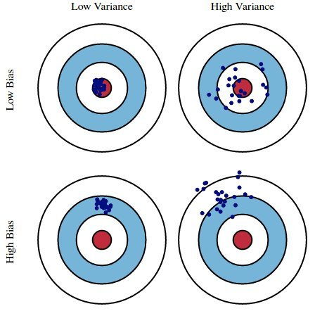
We'd like our models to be in the top left, but in practice that's hard to achieve!
sklearn combine one or more transformers with a single model (estimator), allowing us to perform feature engineering and prediction through a single object.How do we choose the right model complexity, so that our model has the right "balance" between bias and variance?