The wolf classifier
Below, we present a confusion matrix, which summarizes the four possible outcomes of the wolf classifier.

import pandas as pd
import numpy as np
import os

import matplotlib.pyplot as plt
import plotly.express as px
import plotly.graph_objects as go
pd.options.plotting.backend = 'plotly'
TEMPLATE = 'seaborn'

import warnings
warnings.simplefilter('ignore')
Repeat the previous paragraph many, many times.
One night, the shepherd boy sees a real wolf approaching the flock and calls out, "Wolf!" The villagers refuse to be fooled again and stay in their houses. The hungry wolf turns the flock into lamb chops. The town goes hungry. Panic ensues.
Some questions to think about:
Below, we present a confusion matrix, which summarizes the four possible outcomes of the wolf classifier.
When performing binary classification, there are four possible outcomes.
(Note: A "positive prediction" is a prediction of 1, and a "negative prediction" is a prediction of 0.)
| Outcome of Prediction | Definition | True Class |
|---|---|---|
| True positive (TP) ✅ | The predictor correctly predicts the positive class. | P |
| False negative (FN) ❌ | The predictor incorrectly predicts the negative class. | P |
| True negative (TN) ✅ | The predictor correctly predicts the negative class. | N |
| False positive (FP) ❌ | The predictor incorrectly predicts the positive class. | N |
| Predicted Negative | Predicted Positive | |
|---|---|---|
| Actually Negative | TN ✅ | FP ❌ |
| Actually Positive | FN ❌ | TP ✅ |
sklearn's confusion matrices are (but differently than in the wolf example).Note that in the four acronyms – TP, FN, TN, FP – the first letter is whether the prediction is correct, and the second letter is what the prediction is.
The results of 100 UCSD Health COVID tests are given below.
| Predicted Negative | Predicted Positive | |
|---|---|---|
| Actually Negative | TN = 90 ✅ | FP = 1 ❌ |
| Actually Positive | FN = 8 ❌ | TP = 1 ✅ |
🤔 Question: What is the accuracy of the test?
🙋 Answer: $$\text{accuracy} = \frac{TP + TN}{TP + FP + FN + TN} = \frac{1 + 90}{100} = 0.91$$
| Predicted Negative | Predicted Positive | |
|---|---|---|
| Actually Negative | TN = 90 ✅ | FP = 1 ❌ |
| Actually Positive | FN = 8 ❌ | TP = 1 ✅ |
🤔 Question: What proportion of individuals who actually have COVID did the test identify?
🙋 Answer: $\frac{1}{1 + 8} = \frac{1}{9} \approx 0.11$
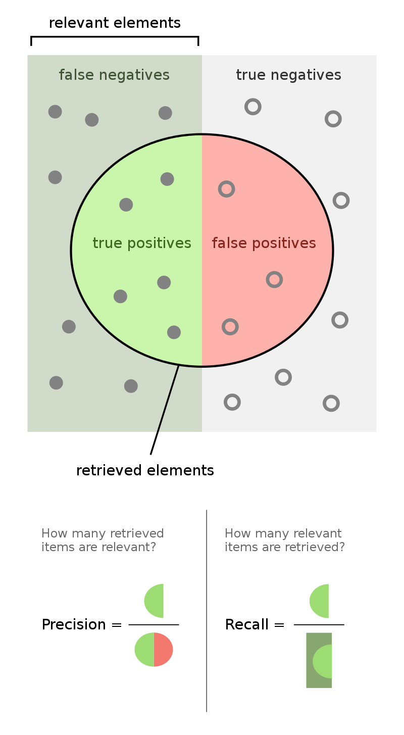
More generally, the recall of a binary classifier is the proportion of actually positive instances that are correctly classified. We'd like this number to be as close to 1 (100%) as possible.
$$\text{recall} = \frac{TP}{\text{# actually positive}} = \frac{TP}{TP + FN}$$To compute recall, look at the bottom (positive) row of the above confusion matrix.
🤔 Question: Can you design a "COVID test" with perfect recall?
🙋 Answer: Yes – just predict that everyone has COVID!
| Predicted Negative | Predicted Positive | |
|---|---|---|
| Actually Negative | TN = 0 ✅ | FP = 91 ❌ |
| Actually Positive | FN = 0 ❌ | TP = 9 ✅ |
Like accuracy, recall on its own is not a perfect metric. Even though the classifier we just created has perfect recall, it has 91 false positives!
| Predicted Negative | Predicted Positive | |
|---|---|---|
| Actually Negative | TN = 0 ✅ | FP = 91 ❌ |
| Actually Positive | FN = 0 ❌ | TP = 9 ✅ |
The precision of a binary classifier is the proportion of predicted positive instances that are correctly classified. We'd like this number to be as close to 1 (100%) as possible.
$$\text{precision} = \frac{TP}{\text{# predicted positive}} = \frac{TP}{TP + FP}$$To compute precision, look at the right (positive) column of the above confusion matrix.
🤔 Question: When might high precision be more important than high recall?
🙋 Answer: For instance, in deciding whether or not someone committed a crime. Here, false positives are really bad – they mean that an innocent person is charged!
🤔 Question: When might high recall be more important than high precision?
🙋 Answer: For instance, in medical tests. Here, false negatives are really bad – they mean that someone's disease goes undetected!
Consider the confusion matrix shown below.
| Predicted Negative | Predicted Positive | |
|---|---|---|
| Actually Negative | TN = 22 ✅ | FP = 2 ❌ |
| Actually Positive | FN = 23 ❌ | TP = 18 ✅ |
What is the accuracy of the above classifier? The precision? The recall?
After calculating all three on your own, click below to see the answers.
The Wisconsin breast cancer dataset (WBCD) is a commonly-used dataset for demonstrating binary classification. It is built into sklearn.datasets.
from sklearn.datasets import load_breast_cancer
loaded = load_breast_cancer() # explore the value of `loaded`!
data = loaded['data']
labels = 1 - loaded['target']
cols = loaded['feature_names']
bc = pd.DataFrame(data, columns=cols)
bc.head()
| mean radius | mean texture | mean perimeter | mean area | mean smoothness | mean compactness | mean concavity | mean concave points | mean symmetry | mean fractal dimension | ... | worst radius | worst texture | worst perimeter | worst area | worst smoothness | worst compactness | worst concavity | worst concave points | worst symmetry | worst fractal dimension | |
|---|---|---|---|---|---|---|---|---|---|---|---|---|---|---|---|---|---|---|---|---|---|
| 0 | 17.99 | 10.38 | 122.80 | 1001.0 | 0.11840 | 0.27760 | 0.3001 | 0.14710 | 0.2419 | 0.07871 | ... | 25.38 | 17.33 | 184.60 | 2019.0 | 0.1622 | 0.6656 | 0.7119 | 0.2654 | 0.4601 | 0.11890 |
| 1 | 20.57 | 17.77 | 132.90 | 1326.0 | 0.08474 | 0.07864 | 0.0869 | 0.07017 | 0.1812 | 0.05667 | ... | 24.99 | 23.41 | 158.80 | 1956.0 | 0.1238 | 0.1866 | 0.2416 | 0.1860 | 0.2750 | 0.08902 |
| 2 | 19.69 | 21.25 | 130.00 | 1203.0 | 0.10960 | 0.15990 | 0.1974 | 0.12790 | 0.2069 | 0.05999 | ... | 23.57 | 25.53 | 152.50 | 1709.0 | 0.1444 | 0.4245 | 0.4504 | 0.2430 | 0.3613 | 0.08758 |
| 3 | 11.42 | 20.38 | 77.58 | 386.1 | 0.14250 | 0.28390 | 0.2414 | 0.10520 | 0.2597 | 0.09744 | ... | 14.91 | 26.50 | 98.87 | 567.7 | 0.2098 | 0.8663 | 0.6869 | 0.2575 | 0.6638 | 0.17300 |
| 4 | 20.29 | 14.34 | 135.10 | 1297.0 | 0.10030 | 0.13280 | 0.1980 | 0.10430 | 0.1809 | 0.05883 | ... | 22.54 | 16.67 | 152.20 | 1575.0 | 0.1374 | 0.2050 | 0.4000 | 0.1625 | 0.2364 | 0.07678 |
5 rows × 30 columns
1 stands for "malignant", i.e. cancerous, and 0 stands for "benign", i.e. safe.
labels[:5]
array([1, 1, 1, 1, 1])
pd.Series(labels).value_counts(normalize=True)
0    0.627417
1    0.372583
dtype: float64
Our goal is to use the features in bc to predict labels.
Logistic regression is a linear classification? technique that builds upon linear regression. It models the probability of belonging to class 1, given a feature vector:
$$P(y = 1 | \vec{x}) = \sigma (\underbrace{w_0 + w_1 x^{(1)} + w_2 x^{(2)} + ... + w_d x^{(d)}}_{\text{linear regression model}})$$Here, $\sigma(t) = \frac{1}{1 + e^{-t}}$ is the sigmoid function; its outputs are between 0 and 1 (which means they can be interpreted as probabilities).
🤔 Question: Suppose our logistic regression model predicts the probability that a tumor is malignant is 0.75. What class do we predict – malignant or benign? What if the predicted probability is 0.3?
🙋 Answer: We have to pick a threshold (e.g. 0.5)!
from sklearn.model_selection import train_test_split
from sklearn.linear_model import LogisticRegression
X_train, X_test, y_train, y_test = train_test_split(bc, labels)
clf = LogisticRegression()
clf.fit(X_train, y_train)
LogisticRegression()
How did clf come up with 1s and 0s?
clf.predict(X_test)
array([0, 0, 0, 0, 0, 0, 0, 1, 0, 0, 1, 0, 0, 1, 1, 0, 0, 0, 0, 1, 0, 0,
       1, 1, 0, 1, 0, 0, 0, 0, 0, 0, 0, 0, 0, 0, 0, 1, 0, 1, 1, 0, 0, 0,
       0, 0, 0, 1, 1, 0, 1, 0, 1, 0, 0, 1, 1, 0, 0, 0, 0, 0, 0, 0, 0, 0,
       1, 0, 1, 1, 0, 0, 0, 0, 0, 0, 0, 0, 1, 1, 0, 0, 0, 1, 1, 1, 1, 1,
       0, 1, 0, 1, 1, 0, 0, 0, 0, 1, 1, 0, 1, 1, 1, 0, 0, 0, 0, 0, 0, 0,
       1, 1, 0, 0, 0, 0, 1, 0, 0, 0, 0, 0, 0, 0, 0, 0, 1, 0, 0, 0, 1, 1,
       1, 0, 1, 0, 0, 0, 0, 1, 0, 1, 1])
It turns out that the predicted labels come from applying a threshold of 0.5 to the predicted probabilities. We can access the predicted probabilities via the predict_proba method:
# [:, 1] refers to the predicted probabilities for class 1
clf.predict_proba(X_test)[:, 1]
array([4.79267883e-01, 2.67827969e-04, 4.76852669e-03, 8.70327442e-03,
       1.21863170e-03, 3.70160949e-03, 3.83147967e-01, 9.99999943e-01,
       4.66204175e-03, 4.97949135e-02, 9.78836837e-01, 5.25592813e-02,
       1.99357043e-02, 1.00000000e+00, 9.99999999e-01, 1.68184647e-01,
       1.32004744e-03, 5.97235870e-02, 6.10571513e-04, 9.94544173e-01,
       1.58385001e-02, 5.96271996e-03, 9.87646468e-01, 9.99999308e-01,
       7.45093008e-02, 9.99999635e-01, 1.34666734e-03, 3.58815186e-03,
       7.25792681e-04, 3.00964858e-02, 7.43892951e-03, 3.90124284e-01,
       3.53632205e-02, 1.83998979e-02, 4.07877069e-02, 4.82118150e-01,
       7.97402959e-02, 5.45118223e-01, 5.39598523e-02, 1.00000000e+00,
       9.99999847e-01, 8.69193761e-04, 1.81118232e-03, 1.40103764e-02,
       8.76509342e-03, 8.51826940e-02, 3.05640094e-04, 9.07055614e-01,
       9.99996854e-01, 1.10164806e-03, 9.99960769e-01, 8.39738072e-04,
       9.99853446e-01, 7.33644323e-03, 7.27749494e-04, 9.99978185e-01,
       9.97342100e-01, 7.33400223e-04, 7.01243148e-02, 1.62988050e-01,
       2.05537549e-01, 2.31460636e-03, 1.17678756e-02, 3.73694738e-02,
       6.55322443e-02, 1.91015031e-02, 9.98132639e-01, 1.79263594e-02,
       9.98735664e-01, 9.99999810e-01, 2.87922004e-03, 3.76868417e-01,
       1.48930825e-02, 3.94710864e-03, 3.11891813e-03, 1.16008076e-02,
       2.43914080e-03, 1.79206056e-02, 1.00000000e+00, 9.99998610e-01,
       4.29458076e-04, 7.37391819e-03, 8.22645940e-03, 1.00000000e+00,
       9.40750871e-01, 9.91048725e-01, 5.32866151e-01, 1.00000000e+00,
       3.44629254e-01, 6.87601229e-01, 3.01413426e-02, 9.97183964e-01,
       9.02357017e-01, 2.28039096e-02, 3.34593997e-02, 1.62305385e-02,
       9.86350687e-03, 9.99838343e-01, 9.99177885e-01, 3.77368576e-03,
       1.00000000e+00, 9.99999999e-01, 1.00000000e+00, 9.69035937e-03,
       4.88720495e-01, 8.66520781e-03, 9.09772555e-04, 3.36368641e-02,
       6.44916191e-03, 6.21002898e-02, 9.35790904e-01, 9.99989435e-01,
       3.55597734e-03, 2.25364520e-02, 5.73787846e-03, 2.52514802e-02,
       9.75565074e-01, 1.50782627e-03, 1.85820922e-01, 2.03491596e-03,
       8.19353870e-03, 4.99770941e-02, 2.83695169e-03, 1.40025315e-01,
       5.60047584e-03, 4.13991392e-03, 9.99999942e-01, 6.34309633e-02,
       1.00997231e-02, 2.86350505e-02, 1.00000000e+00, 1.00000000e+00,
       9.99999968e-01, 2.37308315e-02, 9.99989669e-01, 2.25716024e-02,
       7.61438549e-03, 2.60757316e-01, 2.37460631e-03, 9.99999639e-01,
       4.42059121e-02, 9.99830667e-01, 7.34985866e-01])
Note that our model still has $w^*$s:
clf.intercept_
array([-0.22454193])
clf.coef_
array([[-1.17201122, -0.47956959, -0.05204137,  0.00274439,  0.04403017,
         0.21280417,  0.2934432 ,  0.12392108,  0.06314264,  0.01314701,
        -0.06643895, -0.56592992, -0.23312689,  0.12693186,  0.0031996 ,
         0.04585577,  0.05894403,  0.01518868,  0.01790763,  0.00374143,
        -1.35418505,  0.53133132,  0.158254  ,  0.02015834,  0.07873998,
         0.67181916,  0.81639231,  0.23801492,  0.20903196,  0.06293511]])
Let's see how well our model does on the test set.
from sklearn import metrics
y_pred = clf.predict(X_test)
metrics.accuracy_score(y_test, y_pred)
0.9300699300699301
metrics.precision_score(y_test, y_pred)
0.9782608695652174
metrics.recall_score(y_test, y_pred)
0.8333333333333334
Which metric is more important for this task – precision or recall?
metrics.confusion_matrix(y_test, y_pred)
array([[88,  1],
       [ 9, 45]])
metrics.plot_confusion_matrix(clf, X_test, y_test)
<sklearn.metrics._plot.confusion_matrix.ConfusionMatrixDisplay at 0x7fab2003f460>

🤔 Question: Suppose we choose a threshold higher than 0.5. What will happen to our model's precision and recall?
🙋 Answer: Precision will increase, while recall will decrease*.
Similarly, if we decrease our threshold, our model's precision will decrease, while its recall will increase.
The classification threshold is not actually a hyperparameter of LogisticRegression, because the threshold doesn't change the coefficients ($w^*$s) of the logistic regression model itself (see this article for more details).
As such, if we want to imagine how our predicted classes would change with thresholds other than 0.5, we need to manually threshold.
thresholds = np.arange(0, 1.01, 0.01)
precisions = np.array([])
recalls = np.array([])

for t in thresholds:
    y_pred = clf.predict_proba(X_test)[:, 1] >= t
    precisions = np.append(precisions, metrics.precision_score(y_test, y_pred))
    recalls = np.append(recalls, metrics.recall_score(y_test, y_pred))
Let's visualize the results in plotly, which is interactive.
px.line(x=thresholds, y=precisions,
        labels={'x': 'Threshold', 'y': 'Precision'}, title='Precision vs. Threshold', width=1000, height=600,
        template=TEMPLATE)
px.line(x=thresholds, y=recalls,
        labels={'x': 'Threshold', 'y': 'Recall'}, title='Recall vs. Threshold', width=1000, height=600,
        template=TEMPLATE)
px.line(x=recalls, y=precisions, hover_name=thresholds,
        labels={'x': 'Recall', 'y': 'Precision'}, title='Precision vs. Recall',
        template=TEMPLATE)
The above curve is called a precision-recall (or PR) curve.
🤔 Question: Based on the PR curve above, what threshold would you choose?
If we care equally about a model's precision $PR$ and recall $RE$, we can combine the two using a single metric called the F1-score:
$$\text{F1-score} = \text{harmonic mean}(PR, RE) = 2\frac{PR \cdot RE}{PR + RE}$$pr = metrics.precision_score(y_test, clf.predict(X_test))
re = metrics.recall_score(y_test, clf.predict(X_test))
2 * pr * re / (pr + re)
0.9
metrics.f1_score(y_test, clf.predict(X_test))
0.9
Both F1-score and accuracy are overall measures of a binary classifier's performance. But remember, accuracy is misleading in the presence of class imbalance, and doesn't take into account the kinds of errors the classifier makes.
metrics.accuracy_score(y_test, clf.predict(X_test))
0.9300699300699301
We just scratched the surface! This excellent table from Wikipedia summarizes the many other metrics that exist.
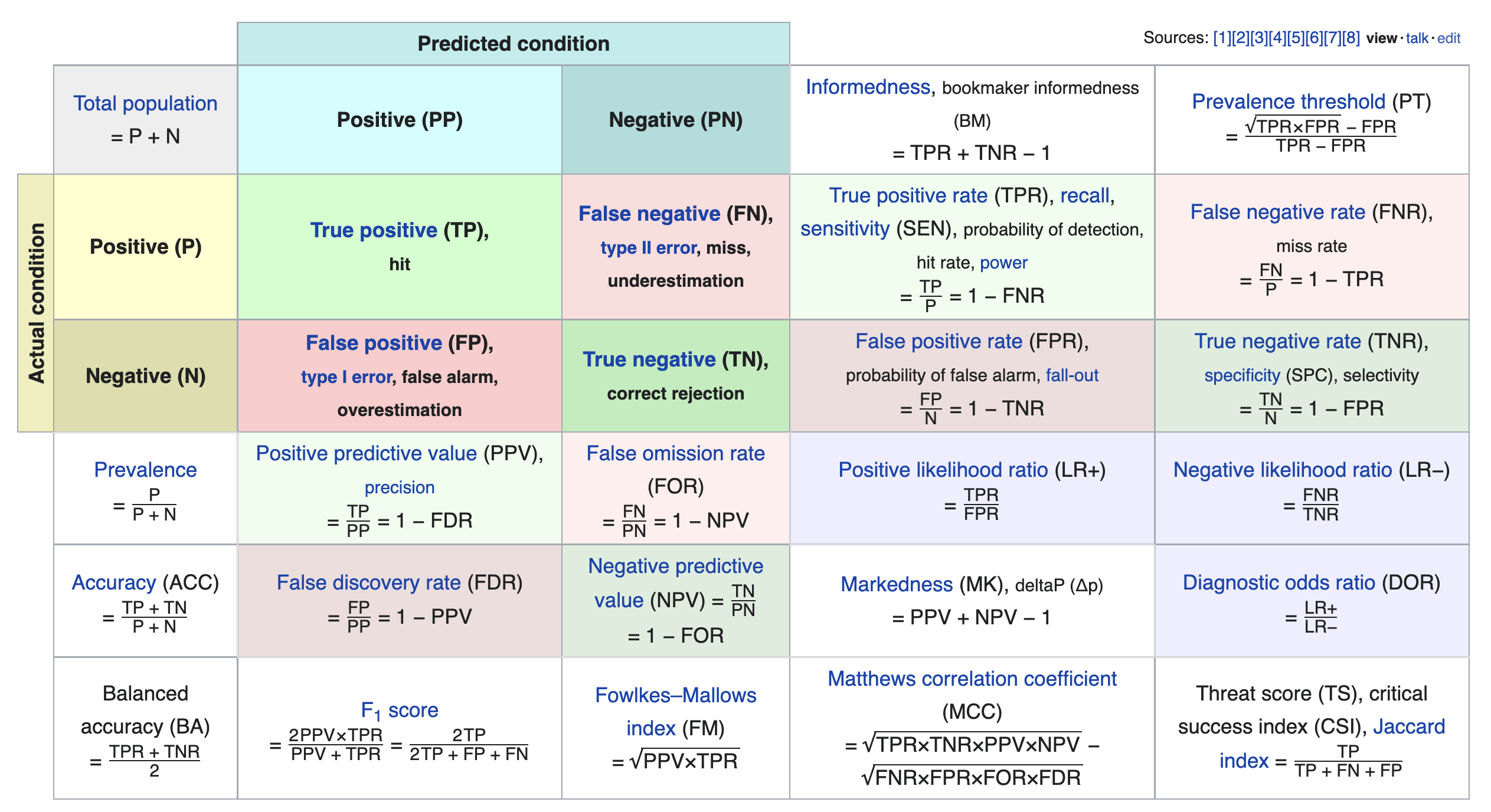
If you're interested in exploring further, a good next metric to look at is true negative rate (i.e. specificity), which is the analogue of recall for true negatives.
Quantifying the fairness of predictive models. Conclusion.