In [1]:
import pandas as pd
import numpy as np
import os

import matplotlib.pyplot as plt
import plotly.express as px
import plotly.graph_objects as go
pd.options.plotting.backend = 'plotly'
TEMPLATE = 'seaborn'

import warnings
warnings.simplefilter('ignore')

Lecture 27 – Fairness, Conclusion

DSC 80, Spring 2023

Agenda

  • Fairness.
  • Parity measures.
  • Example: Loan approval.
  • Parting thoughts.

Fairness

Fairness: why do we care?

  • Sometimes, a model performs better for certain groups than others; in such cases we say the model is unfair.
  • Since ML models are now used in processes that significantly affect human lives, it is important that they are fair!
    • Job applications and college admissions.
    • Criminal sentencing and parole grants.
    • Predictive policing.
    • Credit and loans.

Example: COMPAS and recidivism prediction

COMPAS (Correctional Offender Management Profiling for Alternative Sanctions) is a "black-box" model that estimates the likelihood that someone who has commited a crime will recidivate (commit another crime).


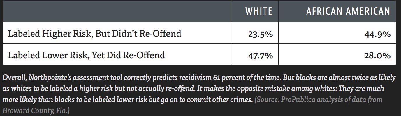
Propublica found that the model's false positive rate is higher for African-Americans than it is for White Americans, and that its false negative rate is lower for African-Americans than it is for White Americans.

Example: Facial recognition

  • The table below comes from a paper that analyzes several "gender classifiers", and shows that popular classifiers perform much worse for women and those with darker skin colors.
  • Police departments are beginning to use these models for surveillance.
  • Self-driving cars use similar models to recognize pedestrians!

Note:

$$PPV = \text{precision} = \frac{TP}{TP+FP},\:\:\:\:\:\: TPR = \text{recall} = \frac{TP}{TP + FN}, \:\:\:\:\:\: FPR = \frac{FP}{FP+TN}$$

How does bias occur?

Remember, our models learn patterns from the training data. Various sources of bias may be present within training data:

  • Training data may not be representative of the population.
    • There may be fewer data points for minority groups, leading to poorer model performance.
  • The features chosen may be more useful in making predictions for certain groups than others.
  • Training data may encode existing human biases.

Example: Gender associations

  • English is not a gendered language – words like "teacher" and "scientist" are not inherently gendered (unlike in, say, French).
  • However, English does have gendered pronouns (e.g. "he", "she").
  • Humans subconsciously associate certain words with certain genders.
  • What gender does English associate the following words with?
soldier, teacher, nurse, doctor, dog, cat, president, nanny

Example: Gender associations

  • Unlike English, Turkish 🇹🇷 does not have gendered pronouns – there is only a single, gender-neutral pronoun ("o").
  • Let's see what happens when we use Google Translate to translate Turkish sentences that should be gender-neutral back to English.
  • Click this link to follow along.
  • Why is this happening?
    • Answer: Google Translate is "trained" on a large corpus of English text, and these associations are present in those English texts.
    • Ideally, the results should contain a gender-neutral singular "they", rather than "he" or "she".

Example: Image searches

A 2015 study examined the image queries of vocations and the gender makeup in the search results. Since 2015, the behavior of Google Images has been improved.

In 2015, a Google Images search for "nurse" returned...

Search for "nurse" now, what do you see?

In 2015, a Google Images search for "doctor" returned...

Search for "doctor" now, what do you see?

Ethics: What gender ratio should we expect in the results?

  • Should it be 50/50?
  • Should it reflect the true gender distribution of those jobs?
  • More generally, what do you expect from your search results?
    • This is a philosophical and ethical question, but one that we need to think about as data scientists.

Excerpts:

"male-dominated professions tend to have even more men

in their results than would be expected if the proportions reflected real-world distributions.

"People’s existing perceptions of gender ratios in occupations

are quite accurate, but that manipulated search results have an effect on perceptions."

How did this unequal representation occur?

  • The training data that Google Images searches from encoded existing biases.
    • While 60% of doctors may be male, 80% of photos (including stock photos) of doctors on the internet may be of male doctors.
  • Models (like PageRank) that "rank" images find the, say, 5 "most relevant" image, not the 5 "most typical" images.

Parity measures

Notation

  • $C$ is a binary classifier.
    • $C \in \{0, 1\}$ is the prediction that the classifier makes.
    • For instance, $C$ may predict whether or not an assignment is plagiarized.
  • $Y \in \{0,1\}$ is the "true" label.
  • $A \in \{0, 1\}$ is a binary attribute of interest.
    • For instance, $A = 1$ may mean that you are a data science major, and $A = 0$ may mean that you are not a data science major.
  • Key idea: A classifier $C$ is "fair" if it performs the same for individuals in group $A$ and individuals outside of group $A$.
    • But what do we mean by "the same"?

Demographic parity

  • A classifier $C$ achieves demographic parity if the proportion of the population for which $C = 1$ is the same both within A and outside A.
$$\mathbb{P}(C=1|A=1) = \mathbb{P}(C=1|A\neq 1)$$
  • The assumption of demographic parity: the proportion of times the classifier predicts 1 is independent of $A$.
  • Example 1: $C$ is a binary classifier that predicts whether or not an essay is plagiarized.
    • Suppose $A$ is "class is a science class".
    • If $C$ achieves demographic parity, then the proportion of the population for which an assignment is predicted to be plagiarized should be equal for science and non-science classes.
  • Example 2: $C$ is a binary classifier that predicts whether an image is of a doctor.
    • Suppose $A$ is "image is of a woman".
    • If $C$ achieves demographic parity, then the proportion of the population for which the classification is "doctor" should be the same for women and non-women.

Accuracy parity

  • Demographic parity is not the only notion of "fairness!"
    • You might expect more instances of plagiarism in non-science classes than you would in science classes; demographic parity says this is unfair but it may not be.
  • A classifier $C$ achieves accuracy parity if the proportion of predictions that are classified correctly is the same both within $A$ and outside of $A$.
$$\mathbb{P}(C=Y|A=1) = \mathbb{P}(C=Y|A\neq 1)$$
  • The assumption of accuracy parity: the classifier's accuracy should be independent of $A$.
  • Example: $C$ is a binary classifier that determines whether someone receives a loan.
    • Suppose $A$ is "age is less than 25".
    • If the classifier is correct, i.e. if $C = Y$, then either $C$ approves the loan and it is paid off, or $C$ denies the loan and it would have defaulted.
    • If $C$ achieves accuracy parity, then the proportion of correctly classified loans should be the same for those under 25 and those over 25.

True positive parity

  • A classifier $C$ achieves true positive parity if the proportion of actually positive individuals that are correctly classified is the same both within $A$ and outside of $A$.
$$\mathbb{P}(C=1|Y=1, A=1) = \mathbb{P}(C=1|Y=1, A\neq 1)$$
  • A more natural way to think of true positive parity is as recall parity – if $C$ achieves true positive parity, its recall should be independent of $A$.

Other measures of parity

  • We've just scratched the surface with measures of parity.
  • Any evaluation metric for a binary classifier can lead to a parity measure – a parity measure requires "similar outcomes" across groups.
    • Precision parity.
    • False positive parity.
  • Note: Many of these parity conditions are impossible to satisfy simultaneously!
    • See DSC 167 for more.

Example: Loan approval

LendingClub

LendingClub is a "peer-to-peer lending company"; they used to publish a dataset describing the loans that they approved (fortunately, we downloaded it while it was available).

  • 'tag': whether loan was repaid in full (1.0) or defaulted (0.0)
  • 'loan_amnt': amount of the loan in dollars
  • 'emp_length': number of years employed
  • 'home_ownership': whether borrower owns (1.0) or rents (0.0)
  • 'inq_last_6mths': number of credit inquiries in last six months
  • 'revol_bal': revolving balance on borrows accounts
  • 'age': age in years of the borrower (protected attribute)
In [2]:
loans = pd.read_csv('data/loan_vars1.csv', index_col=0)
loans.head()
Out[2]:
loan_amnt emp_length home_ownership inq_last_6mths revol_bal age tag
268309 6400.0 0.0 1.0 1.0 899.0 22.0 0.0
301093 10700.0 10.0 1.0 0.0 29411.0 19.0 0.0
1379211 15000.0 10.0 1.0 2.0 9911.0 48.0 0.0
486795 15000.0 10.0 1.0 2.0 15883.0 35.0 0.0
1481134 22775.0 3.0 1.0 0.0 17008.0 39.0 0.0

The total amount of money loaned was over 5 billion dollars!

In [3]:
loans['loan_amnt'].sum()
Out[3]:
5706507225.0
In [4]:
loans.shape[0]
Out[4]:
386772

Predicting 'tag'

Let's build a classifier that predicts whether or not a loan was paid in full. If we were a bank, we could use our trained classifier to determine whether to approve someone for a loan!

In [5]:
from sklearn.model_selection import train_test_split
from sklearn.ensemble import RandomForestClassifier
In [6]:
X = loans.drop('tag', axis=1)
y = loans.tag
X_train, X_test, y_train, y_test = train_test_split(X, y)
In [7]:
clf = RandomForestClassifier(n_estimators=50)
clf.fit(X_train, y_train)
Out[7]:
RandomForestClassifier(n_estimators=50)

Recall, a prediction of 1 means that we predict that the loan will be paid in full.

In [8]:
y_pred = clf.predict(X_test)
y_pred
Out[8]:
array([0., 0., 1., ..., 1., 1., 0.])
In [9]:
clf.score(X_test, y_test)
Out[9]:
0.7141054678208351
In [10]:
from sklearn import metrics
In [11]:
metrics.plot_confusion_matrix(clf, X_test, y_test);

Precision

$$\text{precision} = \frac{TP}{TP+FP}$$

Precision describes the proportion of loans that were approved that would have been paid back.

In [12]:
metrics.precision_score(y_test, y_pred)
Out[12]:
0.7732777155037762

If we subtract the precision from 1, we get the proportion of loans that were approved that would not have been paid back. This is known as the false discovery rate.

$$\frac{FP}{TP + FP} = 1 - \text{precision}$$
In [13]:
1 - metrics.precision_score(y_test, y_pred)
Out[13]:
0.22672228449622378

Recall

$$\text{recall} = \frac{TP}{TP + FN}$$

Recall describes the proportion of loans that would have been paid back that were actually approved.

In [14]:
metrics.recall_score(y_test, y_pred)
Out[14]:
0.7332845417951801

If we subtract the recall from 1, we get the proportion of loans that would have been paid back that were denied. This is known as the false negative rate.

$$\frac{FN}{TP + FN} = 1 - \text{recall}$$
In [15]:
1 - metrics.recall_score(y_test, y_pred)
Out[15]:
0.2667154582048199

From both the perspective of the bank and the lendee, a high false negative rate is bad!

  • The bank left money on the table – the lendee would have paid back the loan, but they weren't approved for a loan.
  • The lendee deserved the loan, but weren't given one.

False negative rate by age

In [16]:
results = X_test
results['age_bracket'] = results['age'].apply(lambda x: 5 * (x // 5 + 1))
results['prediction'] = y_pred
results['tag'] = y_test

(
    results
    .groupby('age_bracket')
    .apply(lambda x: 1 - metrics.recall_score(x['tag'], x['prediction']))
    .plot(kind='bar', title='False Negative Rate by Age Group')
)

Computing parity measures

  • $C$: Our random forest classifier (1 if we approved the loan, 0 if we denied it).
  • $Y$: Whether or not they truly paid off the loan (1) or defaulted (0).
  • $A$: Whether or not they were under 25 (1 if under, 0 if above).
In [17]:
results['is_young'] = (results.age < 25).replace({True: 'young', False: 'old'})

First, let's compute the proportion of loans that were approved in each group. If these two numbers are the same, $C$ achieves demographic parity.

In [18]:
results.groupby('is_young')['prediction'].mean().to_frame()
Out[18]:
prediction
is_young
old 0.685302
young 0.296855

$C$ evidently does not achieve demographic parity – older people are approved for loans far more often! Note that this doesn't factor in whether they were correctly approved or incorrectly approved.

Now, let's compute the accuracy of $C$ in each group. If these two numbers are the same, $C$ achieves accuracy parity.

In [19]:
(
    results
    .groupby('is_young')
    .apply(lambda x: metrics.accuracy_score(x['tag'], x['prediction']))
    .rename('accuracy')
    .to_frame()
)
Out[19]:
accuracy
is_young
old 0.730317
young 0.678910

Hmm... These numbers look much more similar than before!

Is this difference in accuracy significant?

Let's run a permutation test to see if the difference in accuracy is significant.

  • Null Hypothesis: The classifier's accuracy is the same for both young people and old people, and any differences are due to chance.
  • Alternative Hypothesis: The classifier's accuracy is higher for old people.
  • Test statistic: Difference in accuracy (young minus old).
  • Significance level: 0.01.
In [20]:
obs = results.groupby('is_young').apply(lambda x: metrics.accuracy_score(x['tag'], x['prediction'])).diff().iloc[-1]
obs
Out[20]:
-0.051407306793109786
In [21]:
diff_in_acc = []
for _ in range(100):
    s = (
        results[['is_young', 'prediction', 'tag']]
        .assign(is_young=results.is_young.sample(frac=1.0, replace=False).reset_index(drop=True))
        .groupby('is_young')
        .apply(lambda x: metrics.accuracy_score(x['tag'], x['prediction']))
        .diff()
        .iloc[-1]
    )
    
    diff_in_acc.append(s)
In [22]:
fig = pd.Series(diff_in_acc).plot(kind='hist', histnorm='probability', nbins=20,
                            title='Difference in Accuracy (Young - Old)')
fig.add_vline(x=obs, line_color='red')
fig.update_layout(xaxis_range=[-0.1, 0.05])
fig.add_annotation(text='<span style="color:red">Observed Difference in Accuracy</span>', x=-0.075,showarrow=False, y=0.17)

It seems like the difference in accuracy across the two groups is significant, despite being only ~6%. Thus, $C$ likely does not achieve accuracy parity.

Ethical questions of fairness

  • Question: Is it "fair" to deny loans to younger people at a higher rate?
  • One answer: yes!
    • Young people default more often.
    • To have same level of accuracy, we need to deny them loans more often.
  • Other answer: no!
    • Accuracy isn't everything.
    • Younger people need loans to buy houses, pay for school, etc.
    • The bank should be required to take on higher risk; this is the cost of operating in a society.
  • Federal law prevents age from being used as a determining factor in denying a loan.

Not only should we use 'age' to determine whether or not to approve a loan, but we also shouldn't use other features that are strongly correlated with 'age', like 'emp_length'.

In [23]:
loans
Out[23]:
loan_amnt emp_length home_ownership inq_last_6mths revol_bal age tag
268309 6400.0 0.0 1.0 1.0 899.0 22.0 0.0
301093 10700.0 10.0 1.0 0.0 29411.0 19.0 0.0
1379211 15000.0 10.0 1.0 2.0 9911.0 48.0 0.0
486795 15000.0 10.0 1.0 2.0 15883.0 35.0 0.0
1481134 22775.0 3.0 1.0 0.0 17008.0 39.0 0.0
... ... ... ... ... ... ... ...
466121 5000.0 1.0 0.0 0.0 8905.0 23.0 1.0
1354376 2100.0 10.0 1.0 0.0 14740.0 38.0 1.0
1150493 5000.0 1.0 1.0 0.0 3842.0 52.0 1.0
686485 6000.0 10.0 0.0 0.0 6529.0 36.0 1.0
342901 15000.0 8.0 1.0 1.0 16060.0 39.0 1.0

386772 rows × 7 columns

Parting thoughts

Course goals ✅

In this course, you...

  • Practiced translating potentially vague questions into quantitative questions about measurable observations.
  • Learned to reason about 'black-box' processes (e.g. complicated models).
  • Understood computational and statistical implications of working with data.
  • Learned to use real data tools (e.g. love the documentation!).
  • Got a taste of the "life of a data scientist".

Course outcomes ✅

Now, you...

  • Are prepared for internships and data science "take home" interviews!
  • Are ready to create your own portfolio of personal projects.
  • Have the background and maturity to succeed in the upper-division.

Topics covered ✅

We learnt a lot this quarter.

  • Week 1: From BabyPandas to Pandas
  • Week 2: DataFrames
  • Week 3: Messy Data
  • Week 4: Hypothesis and Permutation Testing
  • Week 5: Missingness Mechanisms and Imputation
  • Week 6: Web Scraping, Midterm Exam
  • Week 7: Text Data
  • Week 8: Feature Engineering, Modeling in scikit-learn
  • Week 9: Pipelines and Generalization
  • Week 10: Classifier Evaluation, Fairness Criteria
  • Week 11: Final Exam

Thank you!

  • This course would not have been possible without our 8 tutors and TA: Yuxin Guo, Weiyue Li, Aishani Mohapatra, Costin Smilovici, Yujia Wang, Tiffany Yu, Diego Zavalza and Praveen Nair.

  • Don't be a stranger – our contact information is at dsc80.com/staff!

    • This quarter's course website will remain online permanently at dsc-courses.github.io.
  • Apply to be a tutor in the future! Learn more here.

Good luck on the Final Exam, and enjoy your summer! 🎉