import pandas as pd
import numpy as np
import os

import seaborn as sns
import plotly.express as px
pd.options.plotting.backend = 'plotly'

Lecture 10 – Permutation Testing

DSC 80, Winter 2023

Announcements

• Discussion 3 is today at 5PM.
  • Lab 3 scores and solutions (to non-discussion problems) have been released, or will be shortly.
• Project 2's checkpoint is due tomorrow at 11:59PM, and the full project is due on Thursday, February 9th at 11:59PM.
• Lab 4 (hypothesis and permutation testing) is due on Monday, February 6th at 11:59PM.
• Check out the Grade Report on Gradescope, which details your scores and slip days on most assignments so far.

• I'll be in the CSES "CS Jeopardy" event today from 5-7PM in CSE 1202.
  • I know discussion is from 5-6PM 😢 – if you're interested, you can come after.

Agenda

• Hypothesis testing.
  • Example: Penguin bill lengths 🐧.
• Permutation testing.
  • Great visualization.

Example: Penguins (again!)

(source)

Consider the penguins dataset from a few lectures ago.

penguins = sns.load_dataset('penguins').dropna()
penguins.head()

	species	island	bill_length_mm	bill_depth_mm	flipper_length_mm	body_mass_g	sex
0	Adelie	Torgersen	39.1	18.7	181.0	3750.0	Male
1	Adelie	Torgersen	39.5	17.4	186.0	3800.0	Female
2	Adelie	Torgersen	40.3	18.0	195.0	3250.0	Female
4	Adelie	Torgersen	36.7	19.3	193.0	3450.0	Female
5	Adelie	Torgersen	39.3	20.6	190.0	3650.0	Male

Average bill length by island

penguins.groupby('island')['bill_length_mm'].agg(['mean', 'count'])

	mean	count
island
Biscoe	45.248466	163
Dream	44.221951	123
Torgersen	39.038298	47

It appears that penguins on Torgersen Island have shorter bills on average than penguins on other islands.

Setup

• Null Hypothesis: Island and bill length are not related – the low average bill length of Torgersen Island penguins is due to chance alone.
  • In other words, if we picked 47 penguins randomly from the population of 333 penguins, it is reasonable to see an average this low.

• Alternative Hypothesis: Island and bill length are related – the low average bill length of Torgersen Island penguins is not due to chance alone.

The plan

• The null hypothesis states that the 47 bill lengths of Torgersen Island penguins were drawn uniformly at random from the 333 bill lengths in the population.

• That is, if we repeatedly sampled groups of 47 penguins from the population and computed their mean bill length, it would not be uncommon to see an average bill length this low.

• Plan: Repeatedly sample (without replacement) 47 penguins from the population and compute their average bill length, and see where the Torgersen Island average bill length lies in this distribution.
  • Average bill length is our test statistic.
  • This is not a test statistic we've used in this lecture yet (and this is what separates this example from previous examples).

Simulation

Again, while you could do this with a for-loop (and you can use a for-loop for hypothesis tests in labs and projects), we'll use the faster size approach here.

Instead of using np.random.multinomial, which samples from a categorical distribution, we'll use np.random.choice, which samples from a known sequence of values.

# Draws two samples of size 47 from penguins['bill_length_mm'].
# Question: Why must we sample with replacement here (or, more specifically, in the next cell)?
np.random.choice(penguins['bill_length_mm'], size=(2, 47))

array([[39. , 43.8, 51.5, 52. , 37.6, 50.5, 41.6, 36.2, 51. , 37.6, 36.4,
        37.2, 52. , 43.2, 39.2, 38.5, 40.3, 42.7, 50.2, 48.5, 49.5, 41.1,
        45.2, 46.1, 35.5, 37.6, 52.5, 49.5, 39.6, 51.5, 50.4, 40.5, 44. ,
        44.5, 45.1, 50.2, 45.2, 41.4, 48.8, 40.5, 50.6, 50. , 40.8, 39.2,
        47.2, 51.3, 46.8],
       [42.5, 44.5, 36.6, 45.1, 54.2, 49.4, 36.2, 37.9, 45.2, 49.3, 38.1,
        36.4, 52.2, 39.7, 37.7, 44.9, 52. , 37. , 50.8, 45.1, 47.5, 42.3,
        41.3, 46.8, 42.3, 41. , 55.8, 42.2, 38.8, 48.2, 34.6, 52.7, 39. ,
        45.4, 41.1, 39.8, 36.4, 46.4, 40.9, 37.7, 37.2, 45.5, 42.8, 37.8,
        46.4, 52. , 45. ]])

# Draws 100000 samples of size 47 from penguins['bill_length_mm'].
num_reps = 100_000
averages = np.random.choice(penguins['bill_length_mm'], size=(num_reps, 47)).mean(axis=1)
averages

array([43.9893617 , 43.31914894, 44.25319149, ..., 43.76382979,
       43.5787234 , 43.04680851])

Visualizing the empirical distribution of the test statistic

fig = px.histogram(pd.DataFrame(averages), x=0, nbins=50, histnorm='probability', 
                   title='Empirical Distribution of the Average Bill Length in Samples of Size 47')
fig.add_vline(x=penguins.loc[penguins['island'] == 'Torgersen', 'bill_length_mm'].mean(), line_color='red')

It doesn't look like the average bill length of penguins on Torgersen Island came from the distribution of bill lengths of all penguins in our dataset.

Discussion Question

There is a statistical tool you've learned about that would allow us to find the true probability distribution of the test statistic in this case. What is it?

➡️ Click here to see the answer after you've thought about it.

The Central Limit Theorem (CLT). Recall, the CLT tells us that for any population distribution, the distribution of the sample mean is roughly normal, with the same mean as the population mean. Furthermore, it tells that the standard deviation of the distribution of the sample mean is $\frac{\text{Population SD}}{\sqrt{\text{sample size}}}$. So, the distribution of sample means of samples of size 47 drawn from penguins['bill_length_mm'] is roughly normal with mean penguins['bill_length_mm'].mean() and standard deviation penguins['bill_length_mm'].std(ddof=0) / np.sqrt(47).

Permutation testing

Hypothesis testing vs. permutation testing

"Standard" hypothesis testing helps us answer questions of the form:

I have a population distribution, and I have one sample. Does this sample look like it was drawn from the population?

• Sample: 59 heads and 41 tails. Population: A fair coin.

• Sample: Ethnic distribution of UCSD. Population: Ethnic distribution of California. (Comparing categorical distributions with the TVD.)

• Sample: Sample of Torgersen Island penguins. Population: All 333 penguins. (Comparing a subgroup statistic to a population parameter.)

It does not help us answer questions of the form:

I have two samples, but no information about any population distributions. Do these samples look like they were drawn from the same population?

That's where permutation testing comes in.

Example: Birth weight and smoking 🚬

Note: For familiarity, we'll start with an example from DSC 10. This means we'll move quickly!

Birth weight and smoking 🚬

Let's start by loading in the data.

baby = pd.read_csv(os.path.join('data', 'baby.csv'))
baby.head()

	Birth Weight	Gestational Days	Maternal Age	Maternal Height	Maternal Pregnancy Weight	Maternal Smoker
0	120	284	27	62	100	False
1	113	282	33	64	135	False
2	128	279	28	64	115	True
3	108	282	23	67	125	True
4	136	286	25	62	93	False

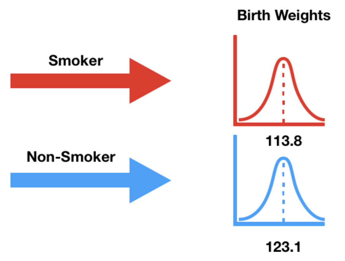
We're only interested in the 'Birth Weight' and 'Maternal Smoker' columns.

baby = baby[['Maternal Smoker', 'Birth Weight']]
baby.head()

	Maternal Smoker	Birth Weight
0	False	120
1	False	113
2	True	128
3	True	108
4	False	136

Note that there are two samples:

• Birth weights of smokers' babies.
• Birth weights of non-smokers' babies.

Exploratory data analysis

How many babies are in each group? What is the average birth weight within each group?

baby.groupby('Maternal Smoker')['Birth Weight'].agg(['mean', 'count'])

	mean	count
Maternal Smoker
False	123.085315	715
True	113.819172	459

Note that 16 ounces are in 1 pound, so the above weights are ~7-8 pounds.

Visualizing birth weight distributions

Below, we draw the distributions of both sets of birth weights.

px.histogram(baby, color='Maternal Smoker', histnorm='probability', marginal='box', 
             title="Birth Weight by Mother's Smoking Status", barmode='overlay', opacity=0.7)

There appears to be a difference, but can it be attributed to random chance?

Hypothesis test setup

• Null Hypothesis: In the population, birth weights of smokers' babies and non-smokers' babies have the same distribution, and the observed differences in our samples are due to random chance.

• Alternative Hypothesis: In the population, smokers' babies have lower birth weights than non-smokers' babies, on average. The observed difference in our samples cannot be explained by random chance alone.

• Issue: We don't know what the population distribution actually is – so how do we draw samples from it?

Null hypothesis: birth weights come from the same distribution

• Our null hypothesis states that "smoker" / "non-smoker" labels have no relationship to birth weight.
• In other words, the "smoker" / "non-smoker" labels may well have been assigned at random.

Alternative hypothesis: birth weights come from different distributions

• Our alternative hypothesis states that the birth weights weights of smokers' babies and non-smokers' babies come from different population distributions.
  • That is, they come from different data generating processes.
• It also states that smokers' babies weigh significantly less.

Choosing a test statistic

We need a test statistic that can measure how different two numerical distributions are.

px.histogram(baby, color='Maternal Smoker', histnorm='probability', marginal='box', 
             title="Birth Weight by Mother's Smoking Status", barmode='overlay', opacity=0.7)

Easiest solution: Difference in group means.

Difference in group means

We'll choose our test statistic to be:

$$\text{mean weight of smokers' babies} - \text{mean weight of non-smokers' babies}$$

We could also compute the non-smokers' mean minus the smokers' mean, too.

group_means = baby.groupby('Maternal Smoker')['Birth Weight'].mean()
group_means

Maternal Smoker
False    123.085315
True     113.819172
Name: Birth Weight, dtype: float64

At first, you may think to use loc with group_means to compute the difference in group means.

group_means.loc[True] - group_means.loc[False]

-9.266142572024918

However, you can also use the diff method.

pd.Series([1, 2, -3]).diff()

0    NaN
1    1.0
2   -5.0
dtype: float64

group_means.diff()

Maternal Smoker
False         NaN
True    -9.266143
Name: Birth Weight, dtype: float64

group_means.diff()[-1]

-9.266142572024918

# If we wanted to do (non-smokers' mean - smokers' mean). 
# Think about why this is the case (hint: it has to do with how the resulting DataFrame after grouping is sorted).
group_means[::-1].diff()[-1]

9.266142572024918

Hypothesis test setup

• Null Hypothesis: In the population, birth weights of smokers' babies and non-smokers' babies have the same distribution, and the observed differences in our samples are due to random chance.

• Alternative Hypothesis: In the population, smokers' babies have lower birth weights than non-smokers' babies, on average. The observed difference in our samples cannot be explained by random chance alone.

• Test Statistic: Difference in group means.

$$\text{mean weight of smokers' babies} - \text{mean weight of non-smokers' babies}$$

• Issue: We don't know what the population distribution actually is – so how do we draw samples from it?
  • This is different from the coin flipping, California ethnicity, and bill length examples, because there the null hypotheses were well-defined probability models.

Implications of the null hypothesis

• Under the null hypothesis, both groups are sampled from the same distribution.
• If this is true, then the group label – 'Maternal Smoker' – has no effect on the birth weight.
• In our dataset, we saw one assignment of True or False to each baby.

baby.head()

	Maternal Smoker	Birth Weight
0	False	120
1	False	113
2	True	128
3	True	108
4	False	136

• Under the null hypothesis, we were just as likely to see any other assignment.

Permutation tests

• In a permutation test, we generate new data by shuffling group labels.
  • In our current example, this involves randomly assigning babies to True or False, while keeping the same number of Trues and Falses as we started with.

• On each shuffle, we'll compute our test statistic (difference in group means).

• If we shuffle many times and compute our test statistic each time, we will approximate the distribution of the test statistic.

• We can them compare our observed statistic to this distribution, as in any other hypothesis test.

Shuffling

• Our goal, by shuffling, is to randomly assign values in the 'Maternal Smoker' column to values in the 'Birth Weight' column.

• We can do this by shuffling either column independently.

• Easiest solution: np.random.permutation.
  • Could also use df.sample, but it's more complicated.

np.random.permutation(baby['Birth Weight'])

array([135,  94, 125, ..., 124, 121, 134])

with_shuffled = baby.assign(Shuffled_Weights=np.random.permutation(baby['Birth Weight']))
with_shuffled.head()

	Maternal Smoker	Birth Weight	Shuffled_Weights
0	False	120	114
1	False	113	139
2	True	128	129
3	True	108	133
4	False	136	114

• Now, we have a new sample of smokers' weights, and a new sample of non-smokers' weights!

• Effectively, we took a random sample of 459 'Birth Weights' and assigned them to the smokers' group, and the remaining 715 to the non-smokers' group.

How close are the means of the shuffled groups?

One benefit of shuffling 'Birth Weight' (instead of 'Maternal Smoker') is that grouping by 'Maternal Smoker' allows us to see all of the following information with a single call to groupby.

group_means = with_shuffled.groupby('Maternal Smoker').mean()
group_means

	Birth Weight	Shuffled_Weights
Maternal Smoker
False	123.085315	119.706294
True	113.819172	119.082789

Let's visualize both pairs of distributions – what do you notice?

for x in ['Birth Weight', 'Shuffled_Weights']:
    fig = px.histogram(with_shuffled, x=x, color='Maternal Smoker', histnorm='probability', marginal='box', 
                 title=f"Using the {x} column (difference in means = {group_means[x].diff().iloc[-1]})", barmode='overlay', opacity=0.7)
    fig.show()

Simulating the empirical distribution of the test statistic

• This was just one random shuffle.

• The question we are trying to answer is, how likely is it that a random shuffle results in two samples where the smokers' mean is at least 9.26 ounces less than the non-smokers' mean?

• To answer this question, we need the distribution of the test statistic. To generate that, we must shuffle many, many times. On each iteration, we must:
  1. Shuffle the weights and store them in a DataFrame.
  2. Compute the test statistic (difference in group means).
  3. Store the result.

n_repetitions = 500

differences = []
for _ in range(n_repetitions):
    
    # Step 1: Shuffle the weights and store them in a DataFrame.
    with_shuffled = baby.assign(Shuffled_Weights=np.random.permutation(baby['Birth Weight']))

    # Step 2: Compute the test statistic.
    # Remember, alphabetically, False comes before True,
    # so this computes True - False.
    group_means = (
        with_shuffled
        .groupby('Maternal Smoker')
        .mean()
        .loc[:, 'Shuffled_Weights']
    )
    difference = group_means.diff().iloc[-1]
    
    # Step 4: Store the result
    differences.append(difference)
    
differences[:10]

[-0.1048036930389884,
 -0.24073921720980707,
 -0.3909837439249202,
 -0.469683257918561,
 1.1758520346755716,
 0.3530843883785053,
 -0.4017154958331446,
 -2.2082270670505864,
 -0.42675625028566344,
 -3.063189969072326]

We already computed the observed statistic earlier, but we compute it again below to keep all of our calculations together.

observed_difference = baby.groupby('Maternal Smoker')['Birth Weight'].mean().diff().iloc[-1]
observed_difference

-9.266142572024918

Conclusion of the test

fig = px.histogram(pd.DataFrame(differences), x=0, nbins=50, histnorm='probability', 
                   title='Empirical Distribution of the Mean Differences in Birth Weights (Smoker - Non-Smoker)')
fig.add_vline(x=observed_difference, line_color='red')
fig.update_layout(xaxis_range=[-15, 15])

• Under the null hypothesis, we rarely see differences as large as 9.26 ounces.

• Therefore, we reject the null hypothesis that the two groups come from the same distribution.

⚠️ Caution!

• We cannot conclude that smoking causes lower birth weight!
• This was an observational study; there may be confounding factors.
  • Maybe smokers are more likely to drink caffeine, and caffeine causes lower birth weight.

Differences between categorical distributions

Example: Married vs. unmarried couples

• We will use data from a study conducted in 2010 by the National Center for Family and Marriage Research.
• The data consists of a national random sample of over 1,000 heterosexual couples who were either married or living together but unmarried.
• Each row corresponds to one person (not one couple).

couples_fp = os.path.join('data', 'married_couples.csv')
couples = pd.read_csv(couples_fp)
couples.head()

	hh_id	gender	mar_status	rel_rating	age	education	hh_income	empl_status	hh_internet
0	0	1	1	1	51	12	14	1	1
1	0	2	1	1	53	9	14	1	1
2	1	1	1	1	57	11	15	1	1
3	1	2	1	1	57	9	15	1	1
4	2	1	1	1	60	12	14	1	1

# What does this expression compute?
couples['hh_id'].value_counts().value_counts()

2    1033
1       2
Name: hh_id, dtype: int64

We won't use all of the columns in the DataFrame.

couples = couples[['mar_status', 'empl_status', 'gender', 'age']]
couples.head()

	mar_status	empl_status	gender	age
0	1	1	1	51
1	1	1	2	53
2	1	1	1	57
3	1	1	2	57
4	1	1	1	60

Cleaning the dataset

The numbers in the DataFrame correspond to the mappings below.

• 'mar_status': 1=married, 2=unmarried.
• 'empl_status': enumerated in the list below.
• 'gender': 1=male, 2=female.
• 'age': person's age in years.

couples.head()

	mar_status	empl_status	gender	age
0	1	1	1	51
1	1	1	2	53
2	1	1	1	57
3	1	1	2	57
4	1	1	1	60

empl = [
    'Working as paid employee',
    'Working, self-employed',
    'Not working - on a temporary layoff from a job',
    'Not working - looking for work',
    'Not working - retired',
    'Not working - disabled',
    'Not working - other'
]

couples = couples.replace({
    'mar_status': {1: 'married', 2: 'unmarried'},
    'gender': {1: 'M', 2: 'F'},
    'empl_status': {(k + 1): empl[k] for k in range(len(empl))}
})

couples.head()

	mar_status	empl_status	gender	age
0	married	Working as paid employee	M	51
1	married	Working as paid employee	F	53
2	married	Working as paid employee	M	57
3	married	Working as paid employee	F	57
4	married	Working as paid employee	M	60

Understanding the couples dataset

• Who is in our dataset? Mostly young people? Mostly married people? Mostly employed people?
• What is the distribution of values in each column?

# For categorical columns, this shows the 10 most common values and their frequencies.
# For numerical columns, this shows the result of calling the .describe() method.
for col in couples:
    if couples[col].dtype == 'object':
        empr = couples[col].value_counts(normalize=True).to_frame().iloc[:10]
    else:
        empr = couples[col].describe().to_frame()
    display(empr)

	mar_status
married	0.717602
unmarried	0.282398

	empl_status
Working as paid employee	0.605899
Not working - other	0.103965
Working, self-employed	0.098646
Not working - looking for work	0.067698
Not working - disabled	0.056576
Not working - retired	0.050774
Not working - on a temporary layoff from a job	0.016441

	gender
M	0.5
F	0.5

	age
count	2068.000000
mean	43.165377
std	11.906982
min	18.000000
25%	33.000000
50%	44.000000
75%	53.000000
max	64.000000

Let's look at the distribution of age separately for married couples and unmarried couples.

px.histogram(couples, x='age', color='mar_status', histnorm='probability', marginal='box',
             barmode='overlay', opacity=0.7)

How are these two distributions different? Why do you think there is a difference?

Understanding employment status in households

• Do married households more often have a stay-at-home spouse?
• Do households with unmarried couples more often have someone looking for work?
• How much does the employment status of the different households vary?

To answer these questions, let's compute the distribution of employment status conditional on household type (married vs. unmarried).

couples.sample(5).head()

	mar_status	empl_status	gender	age
1844	unmarried	Working as paid employee	M	57
1074	married	Working as paid employee	M	34
335	married	Working as paid employee	F	52
1542	married	Working as paid employee	M	35
840	married	Working as paid employee	M	33

# Note that this is a shortcut to picking a column for values and using aggfunc='count'.
empl_cnts = couples.pivot_table(index='empl_status', columns='mar_status', aggfunc='size')
empl_cnts

mar_status	married	unmarried
empl_status
Not working - disabled	72	45
Not working - looking for work	71	69
Not working - on a temporary layoff from a job	21	13
Not working - other	182	33
Not working - retired	94	11
Working as paid employee	906	347
Working, self-employed	138	66

Since there are a different number of married and unmarried couples in the dataset, we can't compare the numbers above directly. We need to convert counts to proportions, separately for married and unmarried couples.

empl_cnts.sum()

mar_status
married      1484
unmarried     584
dtype: int64

cond_distr = empl_cnts / empl_cnts.sum()
cond_distr

mar_status	married	unmarried
empl_status
Not working - disabled	0.048518	0.077055
Not working - looking for work	0.047844	0.118151
Not working - on a temporary layoff from a job	0.014151	0.022260
Not working - other	0.122642	0.056507
Not working - retired	0.063342	0.018836
Working as paid employee	0.610512	0.594178
Working, self-employed	0.092992	0.113014

Both of the columns above sum to 1.

Differences in the distributions

Are the distributions of employment status for married people and for unmarried people who live with their partners different?

Is this difference just due to noise?

cond_distr.plot(kind='barh', title='Distribution of Employment Status, Conditional on Household Type', barmode='group')

Permutation test for household composition

• Null Hypothesis: In the US, the distribution of employment status among those who are married is the same as among those who are unmarried and live with their partners. The difference between the two observed samples is due to chance.

• Alternative Hypothesis: In the US, the distributions of employment status of the two groups are different.

Discussion Question

What is a good test statistic in this case?

Hint: What kind of distributions are we comparing?

Total variation distance

• Whenever we need to compare two categorical distributions, we use the TVD.
  • Recall, the TVD is the sum of the absolute differences in proportions, divided by 2.
• In DSC 10, the only test statistic we ever used in permutation tests was the difference in group means/medians, but the TVD can be used in permutation tests as well.

cond_distr

mar_status	married	unmarried
empl_status
Not working - disabled	0.048518	0.077055
Not working - looking for work	0.047844	0.118151
Not working - on a temporary layoff from a job	0.014151	0.022260
Not working - other	0.122642	0.056507
Not working - retired	0.063342	0.018836
Working as paid employee	0.610512	0.594178
Working, self-employed	0.092992	0.113014

Let's first compute the observed TVD, using our new knowledge of the diff method.

cond_distr.diff(axis=1).iloc[:, -1].abs().sum() / 2

0.1269754089281099

Since we'll need to calculate the TVD repeatedly, let's define a function that computes it.

def tvd_of_groups(df, groups, cats):
    '''groups: the binary column (e.g. married vs. unmarried).
       cats: the categorical column (e.g. employment status).
    '''
    cnts = df.pivot_table(index=cats, columns=groups, aggfunc='size')
    # Normalize each column.
    distr = cnts / cnts.sum()
    # Compute and return the TVD.
    return distr.diff(axis=1).iloc[:, -1].abs().sum() / 2 

# Same result as above.
observed_tvd = tvd_of_groups(couples, groups='mar_status', cats='empl_status')
observed_tvd

0.1269754089281099

Simulation

• Under the null hypothesis, marital status is not related to employment status.
• We can shuffle the marital status column and get an equally-likely dataset.
• On each shuffle, we will compute the TVD.
• Once we have many TVDs, we can ask, how often do we see a difference at least as large as our observed difference?

couples.head()

	mar_status	empl_status	gender	age
0	married	Working as paid employee	M	51
1	married	Working as paid employee	F	53
2	married	Working as paid employee	M	57
3	married	Working as paid employee	F	57
4	married	Working as paid employee	M	60

Here, we'll shuffle marital statuses, though remember, we could shuffle employment statuses too.

couples.assign(shuffled_mar=np.random.permutation(couples['mar_status']))

	mar_status	empl_status	gender	age	shuffled_mar
0	married	Working as paid employee	M	51	married
1	married	Working as paid employee	F	53	married
2	married	Working as paid employee	M	57	unmarried
3	married	Working as paid employee	F	57	unmarried
4	married	Working as paid employee	M	60	married
...	...	...	...	...	...
2063	unmarried	Working as paid employee	F	42	married
2064	unmarried	Working as paid employee	M	60	married
2065	unmarried	Working as paid employee	F	53	unmarried
2066	unmarried	Working as paid employee	M	44	married
2067	unmarried	Working as paid employee	F	42	married

2068 rows × 5 columns

Let's do this repeatedly.

N = 1000
tvds = []

for _ in range(N):
    # Shuffle marital statuses.
    with_shuffled = couples.assign(shuffled_mar=np.random.permutation(couples['mar_status']))
    
    # Compute and store the TVD.
    tvd = tvd_of_groups(with_shuffled, groups='shuffled_mar', cats='empl_status')
    tvds.append(tvd)

Notice that by defining a function that computes our test statistic, our simulation code is much cleaner.

Conclusion of the test

fig = px.histogram(pd.DataFrame(tvds), x=0, nbins=50, histnorm='probability', 
                   title='Empirical Distribution of the TVD')
fig.add_vline(x=observed_tvd, line_color='red')
fig.add_annotation(text=f'<span style="color:red">Observed TVD = {round(observed_tvd, 2)}</span>',
                   x=1.15 * observed_tvd, showarrow=False, y=0.055)

fig.update_layout(xaxis_range=[0, 0.2])
p_95 = np.percentile(tvds, 95)
fig.add_vline(x=p_95, line_color='purple')
annot_text = f'<span style="color:purple">The 95th percentile of our<br>empirical distribution is {round(p_95, 2)}.<br><br>'
annot_text += 'If our observed statistic is to the<br>right of this point, we will reject the null<br>at a 5% <b>significance level</b>.</span>'
fig.add_annotation(text=annot_text, x=1.5 * np.percentile(tvds, 95), showarrow=False, y=0.05)

We reject the null hypothesis that married/unmarried households have similar employment makeups.

We can't say anything about why the employment makeups are different, though!

Discussion Question

In the definition of the TVD, we divide the sum of the absolute differences in proportions between the two distributions by 2.

def tvd(a, b):
    return np.sum(np.abs(a - b)) / 2

Question: If we divided by 200 instead of 2, would we still reject the null hypothesis?

Summary

Summary

• Permutation tests help decide whether two samples came from the same distribution.
• In a permutation test, we simulate data under the null by shuffling either group labels or numerical features.
  • In effect, this randomly assigns individuals to groups.
• If the two distributions are numeric, we use as our test statistic the difference in group means or medians.
• If the two distributions are categorical, we use as our test statistic the total variation distance (TVD).

Next time

Wrap up hypothesis and permutation testing. Revisit missing values.