from dsc80_utils import *
# Pandas Tutor setup
%reload_ext pandas_tutor
%set_pandas_tutor_options {"maxDisplayCols": 8, "nohover": True, "projectorMode": True}
import warnings
warnings.simplefilter(action='ignore', category=FutureWarning)
Announcements 📣
- Lab 2 due tomorrow, Fri, Oct 11.
- Project 1 is due this Tue, Oct 15.
Agenda 📆
- Dataset overview.
- Introduction to
plotly. - Exploratory data analysis and feature types.
- Data cleaning.
- Data quality checks.
- Missing values.
- Transformations and timestamps.
- Modifying structure.
- Investigating student-submitted questions!
Merging
Example: Name categories
The New York Times article from Lecture 1 claims that certain categories of names are becoming more popular. For example:
Forbidden names like Lucifer, Lilith, Kali, and Danger.
Evangelical names like Amen, Savior, Canaan, and Creed.
Mythological names.
It also claims that baby boomer names are becoming less popular.
Let's see if we can verify these claims using data!
Loading in the data
Our first DataFrame, baby, is the same as we saw in Lecture 1. It has one row for every combination of 'Name', 'Sex', and 'Year'.
baby_path = Path('data') / 'baby.csv'
baby = pd.read_csv(baby_path)
baby
Our second DataFrame, nyt, contains the New York Times' categorization of each of several names, based on the aforementioned article.
nyt_path = Path('data') / 'nyt_names.csv'
nyt = pd.read_csv(nyt_path)
nyt
Issue: To find the number of babies born with (for example) forbidden names each year, we need to combine information from both baby and nyt.
Merging
- We want to link rows from
babyandnyttogether whenever the names match up. - This is a merge (
pandasterm), i.e. a join (SQL term). - A merge is appropriate when we have two sources of information about the same individuals that is linked by a common column(s).
- The common column(s) are called the join key.
Example merge
Let's demonstrate on a small subset of baby and nyt.
nyt_small = nyt.iloc[[11, 12, 14]].reset_index(drop=True)

names_to_keep = ['Julius', 'Karen', 'Noah']
baby_small = (baby
 .query("Year == 2020 and Name in @names_to_keep")
 .reset_index(drop=True)
)

dfs_side_by_side(baby_small, nyt_small)
%%pt
baby_small.merge(nyt_small, left_on='Name', right_on='nyt_name')
The merge method
The
mergeDataFrame method joins two DataFrames by columns or indexes.- As mentioned before, "merge" is just the
pandasword for "join."
- As mentioned before, "merge" is just the
When using the
mergemethod, the DataFrame beforemergeis the "left" DataFrame, and the DataFrame passed intomergeis the "right" DataFrame.- In
baby_small.merge(nyt_small),baby_smallis considered the "left" DataFrame andnyt_smallis the "right" DataFrame; the columns from the left DataFrame appear to the left of the columns from right DataFrame.
- In
By default:
- If join keys are not specified, all shared columns between the two DataFrames are used.
- The "type" of join performed is an inner join. This is the only type of join you saw in DSC 10, but there are more, as we'll now see!
Join types: inner joins
%%pt
baby_small.merge(nyt_small, left_on='Name', right_on='nyt_name')
- Note that
'Noah'and'Freya'do not appear in the merged DataFrame. - This is because there is:
- no
'Noah'in the right DataFrame (nyt_small), and - no
'Freya'in the left DataFrame (baby_small).
- no
- The default type of join that
mergeperforms is an inner join, which keeps the intersection of the join keys.

Different join types
We can change the type of join performed by changing the how argument in merge. Let's experiment!
%%pt
# Note the NaNs!
baby_small.merge(nyt_small, left_on='Name', right_on='nyt_name', how='left')
%%pt
baby_small.merge(nyt_small, left_on='Name', right_on='nyt_name', how='right')
%%pt
baby_small.merge(nyt_small, left_on='Name', right_on='nyt_name', how='outer')
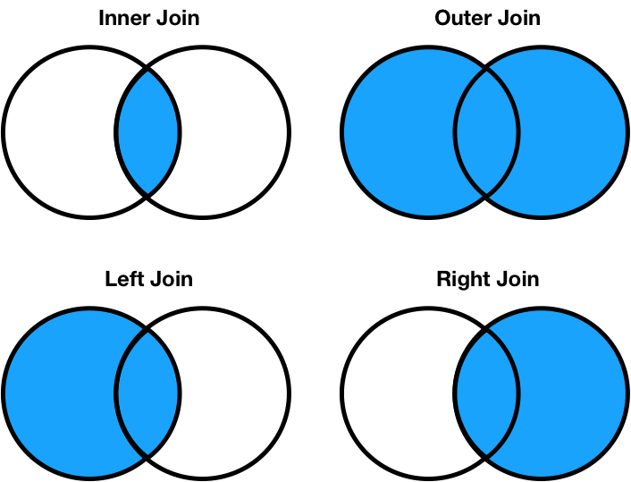
Different join types handle mismatches differently
There are four types of joins.
- Inner: keep only matching keys (intersection).
- Outer: keep all keys in both DataFrames (union).
- Left: keep all keys in the left DataFrame, whether or not they are in the right DataFrame.
- Right: keep all keys in the right DataFrame, whether or not they are in the left DataFrame.
- Note that
a.merge(b, how='left')contains the same information asb.merge(a, how='right'), just in a different order.
- Note that
Notes on the merge method
mergeis flexible – you can merge using a combination of columns, or the index of the DataFrame.- If the two DataFrames have the same column names,
pandaswill add_xand_yto the duplicated column names to avoid having columns with the same name (change these thesuffixesargument). - There is, in fact, a
joinmethod, but it's actually a wrapper aroundmergewith fewer options. - As always, the documentation is your friend!
Lots of pandas operations do an implicit outer join!
pandaswill almost always try to match up index values using an outer join.- It won't tell you that it's doing an outer join, it'll just throw
NaNs in your result!
df1 = pd.DataFrame({'a': [1, 2, 3]}, index=['hello', 'dsc80', 'students'])
df2 = pd.DataFrame({'b': [10, 20, 30]}, index=['dsc80', 'is', 'awesome'])
dfs_side_by_side(df1, df2)
df1['a'] + df2['b']
Many-to-one & many-to-many joins
One-to-one joins
- So far in this lecture, the joins we have worked with are called one-to-one joins.
- Neither the left DataFrame (
baby_small) nor the right DataFrame (nyt_small) contained any duplicates in the join key. - What if there are duplicated join keys, in one or both of the DataFrames we are merging?
# Run this cell to set up the next example.
profs = pd.DataFrame(
[['Sam', 'UCB', 5],
 ['Sam', 'UCSD', 5],
 ['Janine', 'UCSD', 8],
 ['Marina', 'UIC', 7],
 ['Justin', 'OSU', 5],
 ['Soohyun', 'UCSD', 2],
 ['Suraj', 'UCB', 2]],
    columns=['Name', 'School', 'Years']
)

schools = pd.DataFrame({
    'Abr': ['UCSD', 'UCLA', 'UCB', 'UIC'],
    'Full': ['University of California San Diego', 'University of California, Los Angeles', 'University of California, Berkeley', 'University of Illinois Chicago']
})

programs = pd.DataFrame({
    'uni': ['UCSD', 'UCSD', 'UCSD', 'UCB', 'OSU', 'OSU'],
    'dept': ['Math', 'HDSI', 'COGS', 'CS', 'Math', 'CS'],
    'grad_students': [205, 54, 281, 439, 304, 193]
})
Many-to-one joins
- Many-to-one joins are joins where one of the DataFrames contains duplicate values in the join key.
- The resulting DataFrame will preserve those duplicate entries as appropriate.
dfs_side_by_side(profs, schools)
Note that when merging profs and schools, the information from schools is duplicated.
'University of California, San Diego'appears three times.'University of California, Berkeley'appears twice.
%%pt
profs.merge(schools, left_on='School', right_on='Abr', how='left')
Many-to-many joins
Many-to-many joins are joins where both DataFrames have duplicate values in the join key.
dfs_side_by_side(profs, programs)
Before running the following cell, try predicting the number of rows in the output.
%%pt
profs.merge(programs, left_on='School', right_on='uni')
mergestitched together every UCSD row inprofswith every UCSD row inprograms.- Since there were 3 UCSD rows in
profsand 3 inprograms, there are $3 \cdot 3 = 9$ UCSD rows in the output. The same applies for all other schools.
Question 🤔 (Answer at dsc80.com/q)
Code: merge
Fill in the blank so that the last statement evaluates to True.
df = profs.merge(programs, left_on='School', right_on='uni')
df.shape[0] == (____).sum()
Don't use merge (or join) in your solution!
dfs_side_by_side(profs, programs)
# Your code goes here.
Returning back to our original question
Let's find the popularity of baby name categories over time. To start, we'll define a DataFrame that has one row for every combination of 'category' and 'Year'.
cate_counts = (
    baby
    .merge(nyt, left_on='Name', right_on='nyt_name')
    .groupby(['category', 'Year'])
    ['Count']
    .sum()
    .reset_index()
)
cate_counts
# We'll talk about plotting code soon!
import plotly.express as px
fig = px.line(cate_counts, x='Year', y='Count',
              facet_col='category', facet_col_wrap=3,
              facet_row_spacing=0.15,
              width=600, height=400)
fig.update_yaxes(matches=None, showticklabels=False)
fig
Questions? 🤔
Transforming
Transforming values
A transformation results from performing some operation on every element in a sequence, e.g. a Series.
While we haven't discussed it yet in DSC 80, you learned how to transform Series in DSC 10, using the
applymethod.applyis very flexible – it takes in a function, which itself takes in a single value as input and returns a single value.
baby
def number_of_vowels(string):
    return sum(c in 'aeiou' for c in string.lower())

baby['Name'].apply(number_of_vowels)
# Built-in functions work with apply, too.
baby['Name'].apply(len)
The price of apply
Unfortunately, apply runs really slowly!
%%timeit
baby['Name'].apply(number_of_vowels)
%%timeit
res = []
for name in baby['Name']:
    res.append(number_of_vowels(name))
Internally, apply actually just runs a for-loop!
So, when possible – say, when applying arithmetic operations – we should work on Series objects directly and avoid apply!
The price of apply
%%timeit
baby['Year'] // 10 * 10 # Rounds down to the nearest multiple of 10.
%%timeit
baby['Year'].apply(lambda y: y // 10 * 10)
100x slower!
The .str accessor
For string operations, pandas provides a convenient .str accessor.
%%timeit
baby['Name'].str.len()
%%timeit
baby['Name'].apply(len)
It's very convenient and runs about the same speed as apply!
Dataset overview
San Diego food safety
From this article (archive link):
In the last three years, one third of San Diego County restaurants have had at least one major food safety violation.
99% Of San Diego Restaurants Earn ‘A' Grades, Bringing Usefulness of System Into Question
From this article (archive link):
Food held at unsafe temperatures. Employees not washing their hands. Dirty countertops. Vermin in the kitchen. An expired restaurant permit.
Restaurant inspectors for San Diego County found these violations during a routine health inspection of a diner in La Mesa in November 2016. Despite the violations, the restaurant was awarded a score of 90 out of 100, the lowest possible score to achieve an ‘A’ grade.
The data
- We downloaded the data about the 1000 restaurants closest to UCSD from here.
- We had to download the data as JSON files, then process it into DataFrames. You'll learn how to do this soon!
- Until now, you've (largely) been presented with CSV files that
pd.read_csvcould load without any issues. - But there are many different formats and possible issues when loading data in from files.
- See Chapter 8 of Learning DS for more.
- Until now, you've (largely) been presented with CSV files that
rest_path = Path('data') / 'restaurants.csv'
insp_path = Path('data') / 'inspections.csv'
viol_path = Path('data') / 'violations.csv'
rest = pd.read_csv(rest_path)
insp = pd.read_csv(insp_path)
viol = pd.read_csv(viol_path)
Question 🤔 (Answer at dsc80.com/q)
Code: dfs
The first article said that one third of restaurants had at least one major safety violation.
Which DataFrames and columns seem most useful to verify this?
rest.head(2)
rest.columns
insp.head(2)
insp.columns
viol.head(2)
viol.columns
Introduction to plotly
plotly
- We've used
plotlyin lecture briefly, and you even have to use it in Project 1 Question 13, but we haven't yet discussed it formally.
- It's a visualization library that enables interactive visualizations.

Using plotly
There are a few ways we can use plotly:
- Using the
plotly.expresssyntax.plotlyis very flexible, but it can be verbose;plotly.expressallows us to make plots quickly.- See the documentation here – it's very rich (there are good examples for almost everything).
- By setting
pandasplotting backend to'plotly'(by default, it's'matplotlib') and using the DataFrameplotmethod.- The DataFrame
plotmethod is how you created plots in DSC 10!
- The DataFrame
For now, we'll use plotly.express syntax; we've imported it in the dsc80_utils.py file that we import at the top of each lecture notebook.
Initial plots
First, let's look at the distribution of inspection 'score's:
fig = px.histogram(insp['score'])
fig
How about the distribution of average inspection 'score' per 'grade'?
scores = (
    insp[['grade', 'score']]
    .dropna()
    .groupby('grade')
    .mean()
    .reset_index()
)
# x= and y= are columns of scores. Convenient!
px.bar(scores, x='grade', y='score')
# Same as the above!
scores.plot(kind='bar', x='grade', y='score')
Exploratory data analysis and feature types

Exploratory data analysis (EDA)
Historically, data analysis was dominated by formal statistics, including tools like confidence intervals, hypothesis tests, and statistical modeling.
In 1977, John Tukey defined the term exploratory data analysis, which described a philosophy for proceeding about data analysis:
Exploratory data analysis is actively incisive, rather than passively descriptive, with real emphasis on the discovery of the unexpected.
- Practically, EDA involves, among other things, computing summary statistics and drawing plots to understand the nature of the data at hand.
The greatest gains from data come from surprises… The unexpected is best brought to our attention by pictures.
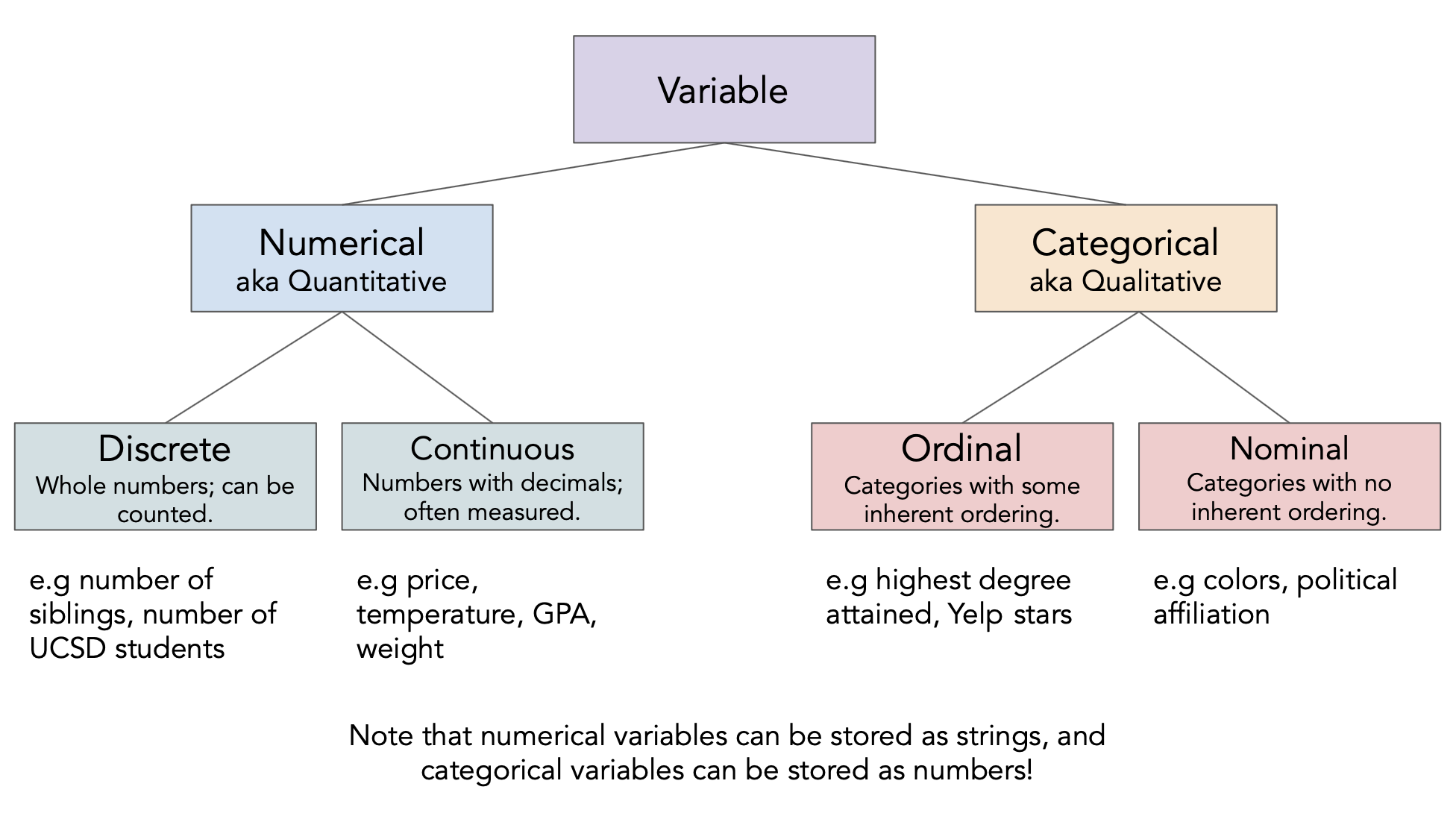
Different feature types
Question 🤔 (Answer at dsc80.com/q)
Code: types
Determine the feature type of each of the following variables.
insp['score']insp['grade']viol['violation_accela']viol['major_violation']rest['business_id']rest['opened_date']
# Your code goes here.
Feature types vs. data types
The data type
pandasuses is not the same as the "data type" we talked about just now!- There's a difference between feature type and computational data type.
Take care when the two don't match up very well!
# pandas stores these as ints, but they're actually nominal.
rest['business_id']
# pandas stores these as strings, but they're actually numeric.
rest['opened_date']
Data cleaning
Four pillars of data cleaning
When loading in a dataset, to clean the data – that is, to prepare it for further analysis – we will:
Perform data quality checks.
Identify and handle missing values.
Perform transformations, including converting time series data to timestamps.
Modify structure as necessary.
Data cleaning: Data quality checks
Data quality checks
We often start an analysis by checking the quality of the data.
- Scope: Do the data match your understanding of the population?
- Measurements and values: Are the values reasonable?
- Relationships: Are related features in agreement?
- Analysis: Which features might be useful in a future analysis?
Scope
Do the data match your understanding of the population?
We were told that we're only looking at the 1000 restaurants closest to UCSD, so the restaurants in rest should agree with that.
rest.sample(5)
Measurements and values
Are the values reasonable?
Do the values in the 'grade' column match what we'd expect grades to look like?
insp['grade'].value_counts()
What kinds of information does the insp DataFrame hold?
insp.info()
What's going on in the 'address' column of rest?
# Are there multiple restaurants with the same address?
rest['address'].value_counts()
# Keeps all rows with duplicate addresses.
(
    rest
    .groupby('address')
    .filter(lambda df: df.shape[0] >= 2)
    .sort_values('address')
)
# Does the same thing as above!
(
    rest[rest.duplicated(subset=['address'], keep=False)]
    .sort_values('address')
)
Relationships
Are related features in agreement?
Do the 'address'es and 'zip' codes in rest match?
rest[['address', 'zip']]
What about the 'score's and 'grade's in insp?
insp[['score', 'grade']]
Analysis
Which features might be useful in a future analysis?
We're most interested in:
- These columns in the
restDataFrame:'business_id','name','address','zip', and'opened_date'. - These columns in the
inspDataFrame:'business_id','inspection_id','score','grade','completed_date', and'status'. - These columns in the
violDataFrame:'inspection_id','violation','major_violation','violation_text', and'violation_accela'.
- These columns in the
Also, let's rename a few columns to make them easier to work with.
💡 Pro-Tip: Using pipe
When we manipulate DataFrames, it's best to define individual functions for each step, then use the pipe method to chain them all together.
The pipe DataFrame method takes in a function, which itself takes in a DataFrame and returns a DataFrame.
- In practice, we would add functions one by one to the top of a notebook, then
pipethem all. - For today, will keep re-running
pipeto show data cleaning process.
def subset_rest(rest):
    return rest[['business_id', 'name', 'address', 'zip', 'opened_date']]

rest = (
    pd.read_csv(rest_path)
    .pipe(subset_rest)
)
rest
# Same as the above – but the above makes it easier to chain more .pipe calls afterwards.
subset_rest(pd.read_csv(rest_path))
Let's use pipe to keep (and rename) the subset of the columns we care about in the other two DataFrames as well.
def subset_insp(insp):
    return (
        insp[['business_id', 'inspection_id', 'score', 'grade', 'completed_date', 'status']]
        .rename(columns={'completed_date': 'date'})
    )

insp = (
    pd.read_csv(insp_path)
    .pipe(subset_insp)
)
def subset_viol(viol):
    return (
        viol[['inspection_id', 'violation', 'major_violation', 'violation_accela']]
        .rename(columns={'violation': 'kind',
                         'major_violation': 'is_major',
                         'violation_accela': 'violation'})
    )

viol = (
    pd.read_csv(viol_path)
    .pipe(subset_viol)
)
Combining the restaurant data
Let's join all three DataFrames together so that we have all the data in a single DataFrame.
def merge_all_restaurant_data():
    return (
        rest
        .merge(insp, on='business_id', how='left')
        .merge(viol, on='inspection_id', how='left')
    )

df = merge_all_restaurant_data()
df
Question 🤔 (Answer at dsc80.com/q)
Code: lefts
Why should the function above use two left joins? What would go wrong if we used other kinds of joins?
Data cleaning: Missing values
Missing values
Next, it's important to check for and handle missing values, as they can have a big effect on your analysis.
insp[['score', 'grade']]
# The proportion of values in each column that are missing.
insp.isna().mean()
# Why are there null values here?
# insp['inspection_id'] and viol['inspection_id'] don't have any null values...
df[df['inspection_id'].isna()]
There are many ways of handling missing values, which we'll cover in an entire lecture next week. But a good first step is to check how many there are!
Data cleaning: Transformations and timestamps
Transformations and timestamps
From last class:
A transformation results from performing some operation on every element in a sequence, e.g. a Series.
It's often useful to look at ways of transforming your data to make it easier to work with.
Type conversions (e.g. changing the string
"$2.99"to the number2.99).Unit conversion (e.g. feet to meters).
Extraction (Getting
'vermin'out of'Vermin Violation Recorded on 10/10/2023').
Creating timestamps
Most commonly, we'll parse dates into pd.Timestamp objects.
# Look at the dtype!
insp['date']
# This magical string tells Python what format the date is in.
# For more info: https://docs.python.org/3/library/datetime.html#strftime-and-strptime-behavior
date_format = '%Y-%m-%d'
pd.to_datetime(insp['date'], format=date_format)
# Another advantage of defining functions is that we can reuse this function
# for the 'opened_date' column in `rest` if we wanted to.
def parse_dates(insp, col):
    date_format = '%Y-%m-%d'
    dates = pd.to_datetime(insp[col], format=date_format)
    return insp.assign(**{col: dates})

insp = (
    pd.read_csv(insp_path)
    .pipe(subset_insp)
    .pipe(parse_dates, 'date')
)

# We should also remake df, since it depends on insp.
# Note that the new insp is used to create df!
df = merge_all_restaurant_data()
# Look at the dtype now!
df['date']
Working with timestamps
- We often want to adjust granularity of timestamps to see overall trends, or seasonality.
- Use the
resamplemethod inpandas(documentation).- Think of it like a version of
groupby, but for timestamps. - For instance,
insp.resample('2W', on='date')separates every two weeks of data into a different group.
- Think of it like a version of
insp.resample('2W', on='date')['score'].mean()
# Where are those numbers coming from?
insp[
    (insp['date'] >= pd.Timestamp('2020-01-05')) &
    (insp['date'] < pd.Timestamp('2020-01-19'))
]['score']
(insp.resample('2W', on='date')
 .size()
 .plot(title='Number of Inspections Over Time')
)
The .dt accessor
Like with Series of strings, pandas has a .dt accessor for properties of timestamps (documentation).
insp['date']
insp['date'].dt.day
insp['date'].dt.dayofweek
dow_counts = insp['date'].dt.dayofweek.value_counts()
fig = px.bar(dow_counts)
fig.update_xaxes(tickvals=np.arange(7), ticktext=['Mon', 'Tues', 'Wed', 'Thurs', 'Fri', 'Sat', 'Sun'])
Data cleaning: Modifying structure
Reshaping DataFrames
We often reshape the DataFrame's structure to make it more convenient for analysis. For example, we can:
Simplify structure by removing columns or taking a set of rows for a particular period of time or geographic area.
- We already did this!
Adjust granularity by aggregating rows together.
- To do this, use
groupby(orresample, if working with timestamps).
- To do this, use
Reshape structure, most commonly by using the DataFrame
meltmethod to un-pivot a dataframe.
Using melt
- The
meltmethod is common enough that we'll give it a special mention. - We'll often encounter pivot tables (esp. from government data), which we call wide data.
- The methods we've introduced work better with long-form data, or tidy data.
- To go from wide to long,
melt.

Example usage of melt
wide_example = pd.DataFrame({
    'Year': [2001, 2002],
    'Jan': [10, 130],
    'Feb': [20, 200],
    'Mar': [30, 340]
}).set_index('Year')
wide_example
wide_example.melt(ignore_index=False)
Exploration
Question 🤔 (Answer at dsc80.com/q)
Code: qs
What questions do you want me to try and answer with the data? I'll start with a single pre-prepared question, and then answer student questions until we run out of time.
Example question: Can we rank restaurants by their number of violations? How about separately for each zip code?
And why would we want to do that? 🤔
Summary, next time
Summary
- Data cleaning is a necessary starting step in data analysis. There are four pillars of data cleaning:
- Quality checks.
- Missing values.
- Transformations and timestamps.
- Modifying structure.
- Approach EDA with an open mind, and draw lots of visualizations.
Next time
Hypothesis and permutation testing. Some of this will be DSC 10 review, but we'll also push further!