from dsc80_utils import *
# Used for plotting examples.
def create_kde_plotly(df, group_col, group1, group2, vals_col, title=''):
fig = ff.create_distplot(
hist_data=[df.loc[df[group_col] == group1, vals_col], df.loc[df[group_col] == group2, vals_col]],
group_labels=[group1, group2],
show_rug=False, show_hist=False,
colors=['#ef553b', '#636efb'],
)
return fig.update_layout(title=title)
Announcements 📣
- Good job on Project 1!
- Project 2 released. Checkpoint due next Tues, Oct 22. Full project due the week after on Oct 29.
- Lab 4 due tomorrow.
- When submitting answers for attendance, copy-paste what you have. Answers that are some variant of "I don't know" will be treated as no submission (because that's not participation). Take your best guess!
Agenda 📆
- Permutation testing
- Missingness mechanisms.
- Why do data go missing?
- Missing by Design.
- Not Missing at Random.
- Missing Completely at Random.
- Missing at Random.
- Formal definitions.
- Identifying missingness mechanisms in data.
Additional resources
These recent lectures have been quite conceptual! Here are a few other places to look for readings; many of these are linked on the course homepage and on the Resources tab of the course website.
- Permutation testing:
- Extra lecture notebook: Fast Permutation Tests.
- Great visualization from Jared Wilber.
- Missingness mechanisms:
Permutation testing
Hypothesis testing vs. permutation testing
- So far, we've used hypothesis tests to answer questions of the form:
I know the population distribution, and I have one sample. Is this sample a likely draw from the population?
- Next, we want to consider questions of the form:
I have two samples, but no information about any population distributions. Do these samples look like they were drawn from different populations? That is, do these two samples look "different"?
Hypothesis testing vs. permutation testing


This framework requires us to be able to draw samples from the baseline population – but what if we don't know that population?
Example: Birth weight and smoking 🚬
For familiarity, we'll start with an example from DSC 10. This means we'll move quickly!
Let's start by loading in the data. Each row corresponds to a mother/baby pair.
baby = pd.read_csv(Path('data') / 'babyweights.csv')
baby
| Birth Weight | Gestational Days | Maternal Age | Maternal Height | Maternal Pregnancy Weight | Maternal Smoker | |
|---|---|---|---|---|---|---|
| 0 | 120 | 284 | 27 | 62 | 100 | False |
| 1 | 113 | 282 | 33 | 64 | 135 | False |
| 2 | 128 | 279 | 28 | 64 | 115 | True |
| ... | ... | ... | ... | ... | ... | ... |
| 1171 | 130 | 291 | 30 | 65 | 150 | True |
| 1172 | 125 | 281 | 21 | 65 | 110 | False |
| 1173 | 117 | 297 | 38 | 65 | 129 | False |
1174 rows × 6 columns
We're only interested in the 'Birth Weight' and 'Maternal Smoker' columns.
baby = baby[['Maternal Smoker', 'Birth Weight']]
baby.head()
| Maternal Smoker | Birth Weight | |
|---|---|---|
| 0 | False | 120 |
| 1 | False | 113 |
| 2 | True | 128 |
| 3 | True | 108 |
| 4 | False | 136 |
Note that there are two samples:
- Birth weights of smokers' babies (rows where
'Maternal Smoker'isTrue). - Birth weights of non-smokers' babies (rows where
'Maternal Smoker'isFalse).
Exploratory data analysis
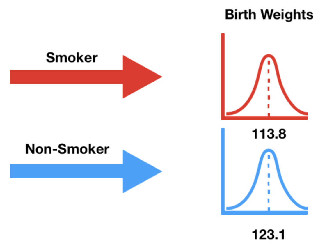
How many babies are in each group? What is the average birth weight within each group?
baby.groupby('Maternal Smoker')['Birth Weight'].agg(['mean', 'count'])
| mean | count | |
|---|---|---|
| Maternal Smoker | ||
| False | 123.09 | 715 |
| True | 113.82 | 459 |
Note that 16 ounces are in 1 pound, so the above weights are ~7-8 pounds.
Visualizing birth weight distributions
Below, we draw the distributions of both sets of birth weights.
fig = px.histogram(baby, color='Maternal Smoker', histnorm='probability', marginal='box',
title="Birth Weight by Mother's Smoking Status", barmode='overlay', opacity=0.7)
fig
There appears to be a difference, but can it be attributed to random chance?
Null hypothesis: birth weights come from the same distribution
- Our null hypothesis states that "smoker" / "non-smoker" labels have no relationship to birth weight.
- In other words, the "smoker" / "non-smoker" labels may well have been assigned at random.

DGP stands for "data generating process" – think of this as another word for population.
Alternative hypothesis: birth weights come from different distributions
- Our alternative hypothesis states that the birth weights weights of smokers' babies and non-smokers' babies come from different population distributions.
- That is, they come from different data generating processes.
- It also states that smokers' babies weigh significantly less.
Choosing a test statistic
We need a test statistic that can measure how different two numerical distributions are.
fig = px.histogram(baby, color='Maternal Smoker', histnorm='probability', marginal='box',
title="Birth Weight by Mother's Smoking Status", barmode='overlay', opacity=0.7)
fig
Easiest solution: Difference in group means.
Difference in group means
We'll choose our test statistic to be:
$$\text{mean weight of smokers' babies} - \text{mean weight of non-smokers' babies}$$
We could also compute the non-smokers' mean minus the smokers' mean, too.
group_means = baby.groupby('Maternal Smoker')['Birth Weight'].mean()
group_means
Maternal Smoker False 123.09 True 113.82 Name: Birth Weight, dtype: float64
Use loc with group_means to compute the difference in group means.
group_means.loc[True] - group_means.loc[False]
np.float64(-9.266142572024918)
Hypothesis test setup
Null Hypothesis: In the population, birth weights of smokers' babies and non-smokers' babies have the same distribution, and the observed differences in our samples are due to random chance.
Alternative Hypothesis: In the population, smokers' babies have lower birth weights than non-smokers' babies, on average. The observed difference in our samples cannot be explained by random chance alone.
Test Statistic: Difference in group means.
$$\text{mean weight of smokers' babies} - \text{mean weight of non-smokers' babies}$$
- Issue: We don't know what the population distribution actually is – so how do we draw samples from it?
- This is different from the coin flipping, and the California ethnicity examples, because there the null hypotheses were well-defined probability models.
Implications of the null hypothesis
- Under the null hypothesis, both groups are sampled from the same distribution.
- If this is true, then the group label –
'Maternal Smoker'– has no effect on the birth weight. - In our dataset, we saw one assignment of
TrueorFalseto each baby.
baby.head()
| Maternal Smoker | Birth Weight | |
|---|---|---|
| 0 | False | 120 |
| 1 | False | 113 |
| 2 | True | 128 |
| 3 | True | 108 |
| 4 | False | 136 |
- Under the null hypothesis, we were just as likely to see any other assignment.
Permutation tests
In a permutation test, we generate new data by shuffling group labels.
- In our current example, this involves randomly assigning babies to
TrueorFalse, while keeping the same number ofTrues andFalses as we started with.
- In our current example, this involves randomly assigning babies to
On each shuffle, we'll compute our test statistic (difference in group means).
If we shuffle many times and compute our test statistic each time, we will approximate the distribution of the test statistic.
We can them compare our observed statistic to this distribution, as in any other hypothesis test.
Shuffling
Our goal, by shuffling, is to randomly assign values in the
'Maternal Smoker'column to values in the'Birth Weight'column.We can do this by shuffling either column independently.
Easiest solution:
np.random.permutation.- We could also use
df.sample, but it's more complicated (and slower).
- We could also use
np.random.permutation(baby['Birth Weight'])
array([ 90, 117, 121, ..., 125, 114, 98])
with_shuffled = baby.assign(Shuffled_Weights=np.random.permutation(baby['Birth Weight']))
with_shuffled.head()
| Maternal Smoker | Birth Weight | Shuffled_Weights | |
|---|---|---|---|
| 0 | False | 120 | 117 |
| 1 | False | 113 | 109 |
| 2 | True | 128 | 114 |
| 3 | True | 108 | 144 |
| 4 | False | 136 | 116 |
Now, we have a new sample of smokers' weights, and a new sample of non-smokers' weights!
Effectively, we took a random sample of 459 'Birth Weights' and assigned them to the smokers' group, and the remaining 715 to the non-smokers' group.
How close are the means of the shuffled groups?
One benefit of shuffling 'Birth Weight' (instead of 'Maternal Smoker') is that grouping by 'Maternal Smoker' allows us to see all of the following information with a single call to groupby.
group_means = with_shuffled.groupby('Maternal Smoker').mean()
group_means
| Birth Weight | Shuffled_Weights | |
|---|---|---|
| Maternal Smoker | ||
| False | 123.09 | 119.12 |
| True | 113.82 | 119.99 |
Let's visualize both pairs of distributions – what do you notice?
for x in ['Birth Weight', 'Shuffled_Weights']:
diff = group_means.loc[True, x] - group_means.loc[False, x]
fig = px.histogram(
with_shuffled, x=x, color='Maternal Smoker', histnorm='probability', marginal='box',
title=f"Using the {x} column <br>(difference in means = {diff:.2f})",
barmode='overlay', opacity=0.7)
fig.update_layout(margin=dict(t=60))
fig.show()
Simulating the empirical distribution of the test statistic
This was just one random shuffle.
The question we are trying to answer is, how likely is it that a random shuffle results in two samples where the difference in group means (smoker minus non-smoker) is $\geq$ 9.26?
To answer this question, we need the distribution of the test statistic. To generate that, we must shuffle many, many times. On each iteration, we must:
- Shuffle the weights and store them in a DataFrame.
- Compute the test statistic (difference in group means).
- Store the result.
n_repetitions = 500
differences = []
for _ in range(n_repetitions):
# Step 1: Shuffle the weights and store them in a DataFrame.
with_shuffled = baby.assign(Shuffled_Weights=np.random.permutation(baby['Birth Weight']))
# Step 2: Compute the test statistic.
# Remember, False (0) comes before True (1),
# so this computes True - False.
group_means = (
with_shuffled
.groupby('Maternal Smoker')
.mean()
.loc[:, 'Shuffled_Weights']
)
difference = group_means.loc[True] - group_means.loc[False]
# Step 4: Store the result
differences.append(difference)
differences[:10]
[np.float64(-0.8703353291588627), np.float64(2.4278897573015144), np.float64(-0.25147096911803146), np.float64(1.1686975334034173), np.float64(0.44967015555249645), np.float64(-0.4196017490135233), np.float64(-0.680741045446922), np.float64(-2.5838383838383834), np.float64(-0.5233420174596546), np.float64(1.5299998476469057)]
We already computed the observed statistic earlier, but we compute it again below to keep all of our calculations together.
mean_weights = baby.groupby('Maternal Smoker')['Birth Weight'].mean()
observed_difference = mean_weights[True] - mean_weights[False]
observed_difference
np.float64(-9.266142572024918)
Conclusion of the test
fig = px.histogram(
pd.DataFrame(differences), x=0, nbins=50, histnorm='probability',
title='Empirical Distribution of the Mean Differences <br> in Birth Weights (Smoker - Non-Smoker)')
fig.add_vline(x=observed_difference, line_color='red')
fig.update_layout(xaxis_range=[-10, 10], margin=dict(t=60))
Under the null hypothesis, we rarely see differences as large as 9.26 ounces.
Therefore, we reject the null hypothesis that the two groups come from the same distribution. That is, the difference between the two samples is statistically significant.
⚠️ Caution!
- We cannot conclude that smoking causes lower birth weight!
- This was an observational study; there may be confounding factors.
- Maybe smokers are more likely to drink caffeine, and caffeine causes lower birth weight.
Hypothesis testing vs. permutation testing
Permutation tests are hypothesis tests!
"Standard" hypothesis tests answer questions of the form:
I have a population distribution, and I have one sample. Does this sample look like it was drawn from the population?
- Permutation tests answer questions of the form:
I have two samples, but no information about any population distributions. Do these samples look like they were drawn from the same population? That is, do these two samples look "similar"?
Question 🤔 (Answer at dsc80.com/q)
Code: dogs22
Taken from the Summer 2022 DSC 10 Final Exam.
Every year, the American Kennel Club holds a Photo Contest for dogs. Eric wants to know whether toy dogs win disproportionately more often than other kinds of dogs. He has collected a sample of 500 dogs that have won the Photo Contest. In his sample, 200 dogs were toy dogs.
Eric also knows the distribution of dog kinds in the population:
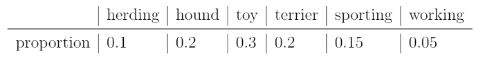
Suppose he has the following null and alternative hypotheses:
- Null Hypothesis: The proportion of toy dogs that win is 0.3.
- Alternative Hypothesis: The proportion of toy dogs that win is greater than 0.3.
Select all the test statistics that Eric can use to conduct his hypothesis.
- A. The proportion of toy dogs in his sample.
- B. The number of toy dogs in his sample.
- C. The absolute difference of the sample proportion of toy dogs and 0.3.
- D. The absolute difference of the sample proportion of toy dogs and 0.5.
- E. The TVD between his sample and the population.
Make sure to check out the "Permutation testing meets TVD" section from last lecture. It has one more example of using a permutation test that you should be familiar with.
Missingness mechanisms
Imperfect data

When studying a problem, we are interested in understanding the true model in nature.
The data generating process is the "real-world" version of the model, that generates the data that we observe.
The recorded data is supposed to "well-represent" the data generating process, and subsequently the true model.
Example: Consider the upcoming Midterm Exam (on May 2, in lecture).
- The exam is meant to be a model of your true knowledge of DSC 80 concepts.
- The data generating process should give us a sense of your true knowledge, but is influenced by the specific questions on the exam, your preparation for the exam, whether or not you are sick on the day of the exam, etc.
- The recorded data consists of the final answers you write on the exam page.
Imperfect data
Problem 1: Your data is not representative, i.e. you have a poor access frame and/or collected a poor sample.
- If the exam only asked questions about
pivot_table, that would not give us an accurate picture of your understanding of DSC 80!
- If the exam only asked questions about
Problem 2: Some of the entries are missing.
- If you left some questions blank, why?
We will focus on the second problem.
Types of missingness
There are four key ways in which values can be missing. It is important to distinguish between these types since in some cases, we can impute (fill in) the missing data.
- Missing by design (MD).
- Not missing at random (NMAR).
- Also called "non-ignorable" (NI).
- Missing at random (MAR).
- Missing completely at random (MCAR).
Missing by design (MD)
Values in a column are missing by design if:
- the designers of the data collection process intentionally decided to not collect data in that column,
- because it can be recovered from other columns.
If you can determine whether a value is missing solely using other columns, then the data is missing by design.
- For example:
'Age4'is missing if and only if'Number of People'is less than 4.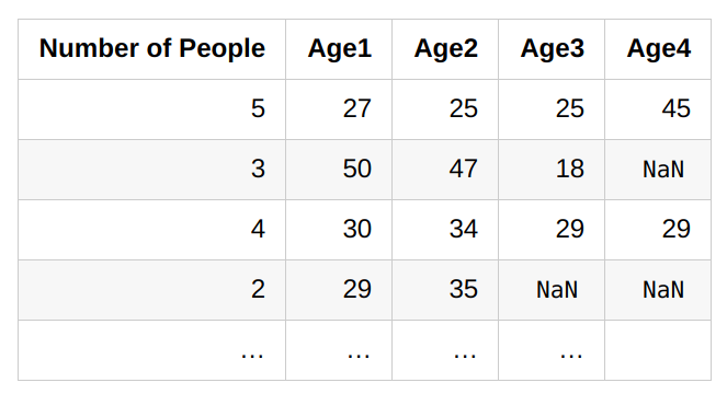
- For example:
Refer to this StackExchange link for more examples.
Missing by design
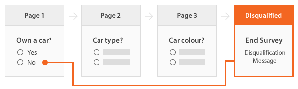
Example: 'Car Type?' and 'Car Colour?' are missing if and only if 'Own a car?' is 'No'.
Other types of missingness
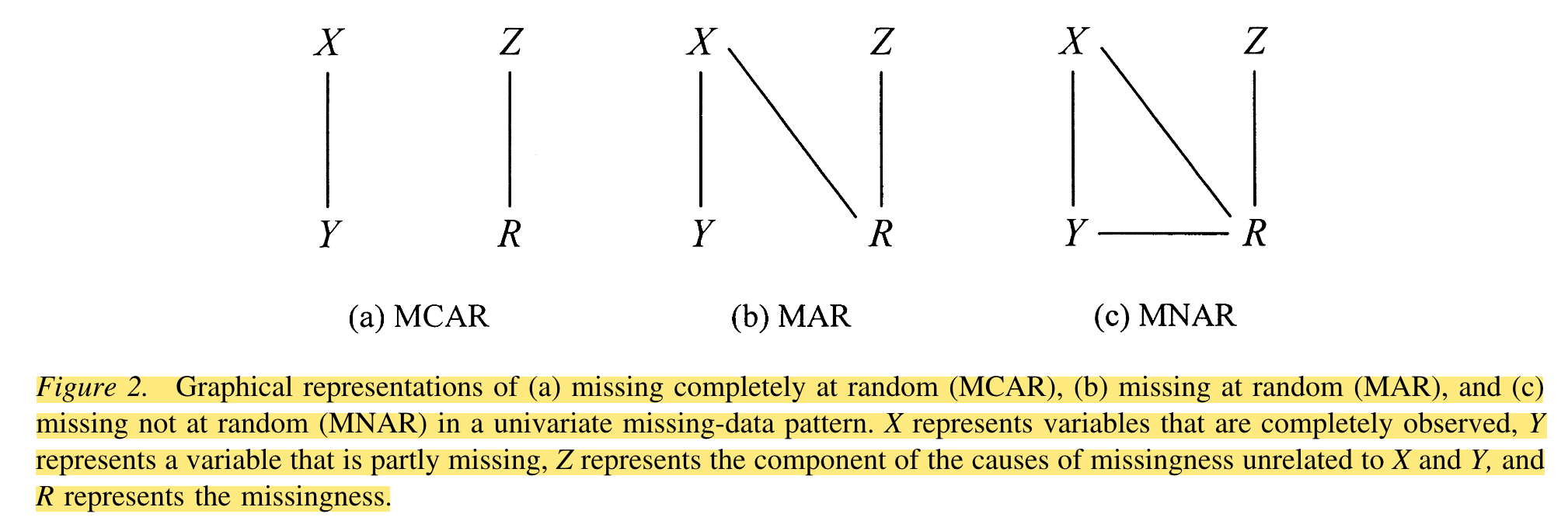
Not missing at random (NMAR).
- The chance that a value is missing depends on the actual missing value!
Missing completely at random (MCAR).
- The chance that a value is missing is completely independent of
- other columns, and
- the actual missing value.
- The chance that a value is missing is completely independent of
Missing at random (MAR).
- The chance that a value is missing depends on other columns, but not the actual missing value itself.
- If a column is MAR, then it is MCAR when conditioned on some set of other columns.
Mom... the dog ate my data! 🐶
Consider the following (contrived) example:
- We survey 100 people for their favorite color and birth month.
- We write their answers on index cards.
- On the left side, we write colors.
- On the right side, we write birth months 📆.
- A silly dog takes the top 10 cards from the stack and chews off the right side (birth months).
- Now ten people are missing birth months!
Question 🤔 (Answer at dsc80.com/q)
Code: cards
We are now missing birth months for the first 10 people we surveyed. What is the missingness mechanism for birth months if:
- Cards were sorted by favorite color?
- Cards were sorted by birth month?
- Cards were shuffled?
Remember:
- Not missing at random (NMAR): The chance that a value is missing depends on the actual missing value!
- Missing at random (MAR): The chance that a value is missing depends on other columns, but not the actual missing value itself.
- Missing completely at random (MCAR): The chance that a value is missing is completely independent of other columns and the actual missing value.
The real world is messy! 🌎
- In our contrived example, the distinction between NMAR, MAR, and MCAR was relatively clear.
- However, in more practical examples, it can be hard to distinguish between types of missingness.
- Domain knowledge is often needed to understand why values might be missing.
Not missing at random (NMAR)
Data is NMAR if the chance that a value is missing depends on the actual missing value!
- It could also depend on other columns.
Another term for NMAR is "non-ignorable" – the fact that data is missing is data in and of itself that we cannot ignore.
Example: A person doesn't take a drug test because they took drugs the day before.
Example: On an employment survey, people with really high incomes may be less likely to report their income.
- If we ignore missingness and compute the mean salary, our result will be biased low!
When data is NMAR, we must reason about why the data is missing using domain expertise on the data generating process – the other columns in our data won't help.
Missing completely at random (MCAR)
Data is MCAR if the chance that a value is missing is completely independent of other columns and the actual missing value.
Example: After the Midterm Exam, I accidentally spill boba on the top of the stack. Assuming that the exams are in a random order, the exam scores that are lost due to this still will be MCAR. (Hopefully this doesn't happen!)

Missing at random (MAR)
Data is MAR if the chance that a value is missing depends on other columns, but not the actual missing value itself.
Example: People who work in the service industry may be less likely to report their income.
- If you look at service industry workers only, there is no pattern to the missingness of income (MCAR).
- If you look at corporate workers only, there is no pattern to the missingness of income (MCAR).
- Within each industry, missingness is MCAR, but overall, it is MAR, since the missingness of income depends on industry.
- Example: An elementary school teacher keeps track of the health conditions of each student in their class. One day, a student doesn't show up for a test because they are at the hospital.
- The fact that their test score is missing has nothing to do with the test score itself.
- But the teacher could have predicted that the score would have been missing given the other information they had about the student.
Isn't everything NMAR? 🤔
You can argue that many of these examples are NMAR, by arguing that the missingness depends on the value of the data that is missing.
- For example, if a student is hospitalized, they may have lots of health problems and may not have spent much time on school, leading to their test scores being worse.
Fair point, but with that logic almost everything is NMAR. What we really care about is the main reason data is missing.
If the other columns mostly explain the missing value and missingness, treat it as MAR.
In other words, accounting for potential confounding variables makes NMAR data more like MAR.
- This is a big part of experimental design.
Flowchart
A good strategy is to assess missingness in the following order.
Question 🤔 (Answer at dsc80.com/q)
Code: missings
In each of the following examples, decide whether the missing data are likely to be MD, NMAR, MAR, or MCAR:
- A table for a medical study has columns for
'gender'and'age'.'age'has missing values. - Measurements from the Hubble Space Telescope are dropped during transmission.
- A table has a single column,
'self-reported education level', which contains missing values. - A table of grades contains three columns,
'Version 1','Version 2', and'Version 3'. $\frac{2}{3}$ of the entries in the table areNaN.
Why do we care again?
- If a dataset contains missing values, it is likely not an accurate picture of the data generating process.
- By identifying missingness mechanisms, we can best fill in missing values, to gain a better understanding of the DGP.
Question 🤔 (Answer at dsc80.com/q)
Code: q07
Send in one topic covered so far (can be from this lecture or any previous one) that you feel unsure about.
Formal definitions
We won't spend much time on these in lecture, but you may find them helpful.
Suppose we have:
- A dataset $Y$ with observed values $Y_{obs}$ and missing values $Y_{mis}$.
Data is missing completely at random (MCAR) if
$$\text{P}(\text{data is present} \: | \: Y_{obs}, Y_{mis}) = \text{P}(\text{data is present})$$
In other words, the chance that a missing value appears doesn't depend on our data (missing or otherwise).
Data is missing at random (MAR) if
$$\text{P}(\text{data is present} \: | \: Y_{obs}, Y_{mis}) = \text{P}(\text{data is present} \: | \: Y_{obs})$$
That is, MAR data is actually MCAR, conditional on $Y_{obs}$.
Data is not missing at random (NMAR) if
$$\text{P}(\text{data is present} \: | \: Y_{obs}, Y_{mis})$$
cannot be simplified. That is, in NMAR data, missingness is dependent on the missing value itself.
A diagram (Sam will annotate)
Identifying missingness mechanisms in data
Identifying missingness mechanisms in data
- Suppose I believe that the missingness mechanism of a column is NMAR, MAR, or MCAR.
- I've ruled out missing by design (a good first step).
- Can I check whether this is true, by looking at the data?
Assessing NMAR
We can't determine if data is NMAR just by looking at the data, as whether or not data is NMAR depends on the unobserved data.
To establish if data is NMAR, we must:
- reason about the data generating process, or
- collect more data.
Example: Consider a dataset of survey data of students' self-reported happiness. The data contains PIDs and happiness scores; nothing else. Some happiness scores are missing. Are happiness scores likely NMAR?
Assessing MAR
Data are MAR if the missingness only depends on observed data.
After reasoning about the data generating process, if you assume that data is not NMAR, then it must be either MAR or MCAR.
The more columns we have in our dataset that are correlated with missingness, the "weaker the NMAR effect" is.
- Adding more columns -> controlling for more variables -> moving from NMAR to MAR.
- Example: With no other columns, income in a census is NMAR. But once we look at location, education, and occupation, incomes are closer to being MAR.
Deciding between MCAR and MAR
For data to be MCAR, the chance that values are missing should not depend on any other column or the values themselves.
Example: Consider a dataset of phones, in which we store the screen size and price of each phone. Some prices are missing.
| Phone | Screen Size | Price |
|---|---|---|
| iPhone 15 | 6.06 | 999 |
| Galaxy Z Fold5 | 7.6 | NaN |
| OnePlus 12R | 6.7 | 499 |
| iPhone 14 Pro Max | 6.68 | NaN |
If prices are MCAR, then the distribution of screen size should be the same for:
- phones whose prices are missing, and
- phones whose prices aren't missing.
We can use a permutation test to decide between MAR and MCAR! We are asking the question, did these two samples come from the same underlying distribution?
Deciding between MCAR and MAR
Suppose you have a DataFrame with columns named $\text{col}_1$, $\text{col}_2$, ..., $\text{col}_k$, and want to test whether values in $\text{col}_X$ are MCAR. To test whether $\text{col}_X$'s missingness is independent of all other columns in the DataFrame:
For $i = 1, 2, ..., k$, where $i \neq X$:
Look at the distribution of $\text{col}_i$ when $\text{col}_X$ is missing.
Look at the distribution of $\text{col}_i$ when $\text{col}_X$ is not missing.
Check if these two distributions are the same. (What do we mean by "the same"?)
If so, then $\text{col}_X$'s missingness doesn't depend on $\text{col}_i$.
If not, then $\text{col}_X$ is MAR dependent on $\text{col}_i$.
If all pairs of distributions were the same, then $\text{col}_X$ is MCAR.
Example: Heights
- Let's load in Galton's dataset containing the heights of adult children and their parents (which you may have seen in DSC 10).
- The dataset does not contain any missing values – we will artifically introduce missing values such that the values are MCAR, for illustration.
heights_path = Path('data') / 'midparent.csv'
heights = (pd.read_csv(heights_path)
.rename(columns={'childHeight': 'child'})
[['father', 'mother', 'gender', 'child']])
heights.head()
| father | mother | gender | child | |
|---|---|---|---|---|
| 0 | 78.5 | 67.0 | male | 73.2 |
| 1 | 78.5 | 67.0 | female | 69.2 |
| 2 | 78.5 | 67.0 | female | 69.0 |
| 3 | 78.5 | 67.0 | female | 69.0 |
| 4 | 75.5 | 66.5 | male | 73.5 |
Proof that there aren't currently any missing values in heights:
heights.isna().sum()
father 0 mother 0 gender 0 child 0 dtype: int64
We have three numerical columns – 'father', 'mother', and 'child'. Let's visualize them simultaneously.
fig = px.scatter_matrix(heights.drop(columns=['gender']))
fig
Simulating MCAR data
- We will make
'child'MCAR by taking a random subset ofheightsand setting the corresponding'child'heights tonp.NaN. - This is equivalent to flipping a (biased) coin for each row.
- If heads, we delete the
'child'height.
- If heads, we delete the
- You will not do this in practice!
np.random.seed(42) # So that we get the same results each time (for lecture).
heights_mcar = heights.copy()
idx = heights_mcar.sample(frac=0.3).index
heights_mcar.loc[idx, 'child'] = np.nan
heights_mcar.head(10)
| father | mother | gender | child | |
|---|---|---|---|---|
| 0 | 78.5 | 67.0 | male | 73.2 |
| 1 | 78.5 | 67.0 | female | 69.2 |
| 2 | 78.5 | 67.0 | female | NaN |
| ... | ... | ... | ... | ... |
| 7 | 75.5 | 66.5 | female | NaN |
| 8 | 75.0 | 64.0 | male | 71.0 |
| 9 | 75.0 | 64.0 | female | 68.0 |
10 rows × 4 columns
heights_mcar.isna().mean()
father 0.0 mother 0.0 gender 0.0 child 0.3 dtype: float64
Verifying that child heights are MCAR in heights_mcar
- Each row of
heights_mcarbelongs to one of two groups:- Group 1:
'child'is missing. - Group 2:
'child'is not missing.
- Group 1:
heights_mcar['child_missing'] = heights_mcar['child'].isna()
heights_mcar.head()
| father | mother | gender | child | child_missing | |
|---|---|---|---|---|---|
| 0 | 78.5 | 67.0 | male | 73.2 | False |
| 1 | 78.5 | 67.0 | female | 69.2 | False |
| 2 | 78.5 | 67.0 | female | NaN | True |
| 3 | 78.5 | 67.0 | female | 69.0 | False |
| 4 | 75.5 | 66.5 | male | 73.5 | False |
- We need to look at the distributions of every other column –
'gender','mother', and'father'– separately for these two groups, and check to see if they are similar.
Comparing null and non-null 'child' distributions for 'gender'
gender_dist = (
heights_mcar
.assign(child_missing=heights_mcar['child'].isna())
.pivot_table(index='gender', columns='child_missing', aggfunc='size')
)
# Added just to make the resulting pivot table easier to read.
gender_dist.columns = ['child_missing = False', 'child_missing = True']
gender_dist = gender_dist / gender_dist.sum()
gender_dist
| child_missing = False | child_missing = True | |
|---|---|---|
| gender | ||
| female | 0.49 | 0.48 |
| male | 0.51 | 0.52 |
- Note that here, each column is a separate distribution that adds to 1.
- The two columns look similar, which is evidence that
'child''s missingness does not depend on'gender'.- Knowing that the child is
'female'doesn't make it any more or less likely that their height is missing than knowing if the child is'male'.
- Knowing that the child is
Comparing null and non-null 'child' distributions for 'gender'
In the previous slide, we saw that the distribution of
'gender'is similar whether or not'child'is missing.To make precise what we mean by "similar", we can run a permutation test. We are comparing two distributions:
- The distribution of
'gender'when'child'is missing. - The distribution of
'gender'when'child'is not missing.
- The distribution of
What test statistic do we use to compare categorical distributions?
gender_dist.plot(kind='barh', title='Gender by Missingness of Child Height', barmode='group')
To measure the "distance" between two categorical distributions, we use the total variation distance.
Note that with only two categories, the TVD is the same as the absolute difference in proportions for either category.
Simulation
The code to run our simulation largely looks the same as in previous permutation tests. Remember, we are comparing two distributions:
- The distribution of 'gender' when 'child' is missing.
- The distribution of 'gender' when 'child' is not missing.
n_repetitions = 500
shuffled = heights_mcar.copy()
tvds = []
for _ in range(n_repetitions):
# Shuffling genders.
# Note that we are assigning back to the same DataFrame for performance reasons;
# see https://dsc80.com/resources/lectures/lec07/lec07-fast-permutation-tests.html.
shuffled['gender'] = np.random.permutation(shuffled['gender'])
# Computing and storing the TVD.
pivoted = (
shuffled
.pivot_table(index='gender', columns='child_missing', aggfunc='size')
)
pivoted = pivoted / pivoted.sum()
tvd = pivoted.diff(axis=1).iloc[:, -1].abs().sum() / 2
tvds.append(tvd)
observed_tvd = gender_dist.diff(axis=1).iloc[:, -1].abs().sum() / 2
observed_tvd
np.float64(0.009196155526430771)
Results
fig = px.histogram(pd.DataFrame(tvds), x=0, nbins=50, histnorm='probability',
title='Empirical Distribution of the TVD')
fig.add_vline(x=observed_tvd, line_color='red', line_width=2, opacity=1)
fig.add_annotation(text=f'<span style="color:red">Observed TVD = {round(observed_tvd, 2)}</span>',
x=2.5 * observed_tvd, showarrow=False, y=0.16)
fig.update_layout(yaxis_range=[0, 0.2])
(np.array(tvds) >= observed_tvd).mean()
np.float64(0.838)
- We fail to reject the null.
- Recall, the null stated that the distribution of
'gender'when'child'is missing is the same as the distribution of'gender'when'child'is not missing. - Hence, this test does not provide evidence that the missingness in the
'child'column is dependent on'gender'.
Comparing null and non-null 'child' distributions for 'father'
We again must compare two distributions:
- The distribution of
'father'when'child'is missing. - The distribution of
'father'when'child'is not missing.
- The distribution of
If the distributions are similar, we conclude that the missingness of
'child'is not dependent on the height of the'father'.We can again use a permutation test.
px.histogram(heights_mcar, x='father', color='child_missing', histnorm='probability', marginal='box',
title="Father's Height by Missingness of Child Height", barmode='overlay', opacity=0.7)
We can visualize numerical distributions with histograms, or with kernel density estimates. (See the definition of create_kde_plotly at the top of the notebook if you're curious as to how these are created.)
create_kde_plotly(heights_mcar, 'child_missing', True, False, 'father',
"Father's Height by Missingness of Child Height")
Concluding that 'child' is MCAR
We need to run three permutation tests – one for each column in
heights_mcarother than'child'.For every other column, if we fail to reject the null that the distribution of the column when
'child'is missing is the same as the distribution of the column when'child'is not missing, then we can conclude'child'is MCAR.- In such a case, its missingness is not tied to any other columns.
- For instance, children with shorter fathers are not any more likely to have missing heights than children with taller fathers.
Summary, next time
Summary
- Refer to the Flowchart for an overview of the four missingness mechanisms.
- We can use permutation tests to verify if a column is MAR vs. MCAR.
- Create two groups: one where values in a column are missing, and another where values in a column aren't missing.
- To test the missingness of column X:
- For every other column, test the null hypothesis "the distribution of (other column) is the same when column X is missing and when column X is not missing."
- If you fail to reject the null, then column X's missingness does not depend on (other column).
- If you reject the null, then column X is MAR dependent on (other column).
- If you fail to reject the null for all other columns, then column X is MCAR!
Next time
- More examples of deciding between MCAR and MAR using permutation tests.
- For instance, we'll simulate MAR data and see if we can detect whether it is MAR.
- We'll also learn about a new test statistic for measuring the similarity between two categorical distributions.
- Imputation: given that we know a column's missingness mechanism, how do we fill in its missing values?