from dsc80_utils import *
Announcements 📣
- Midterm Survey due tonight: https://forms.gle/8pMeYeHk6ktLa4867
- If ≥80% of the class fills it out, everyone will get +1% EC on the midterm.
- Lab 6 is due tomorrow.
- The Final Project will be released next week.
Agenda 📆
- Last bits of TF-IDF.
- Modeling.
- Case study: Restaurant tips 🧑🍳.
- Regression in
sklearn. - Announcement about HDSI career services.
Conceptually, today will mostly be review from DSC 40A, but we'll introduce a few new practical tools that we'll build upon next week.
State of the Union addresses
from pathlib import Path
sotu_txt = Path('data') / 'stateoftheunion1790-2023.txt'
sotu = sotu_txt.read_text()
speeches = sotu.split('\n***\n')[1:]
import re
def extract_struct(speech):
L = speech.strip().split('\n', maxsplit=3)
L[3] = re.sub(r"[^A-Za-z' ]", ' ', L[3]).lower()
return dict(zip(['speech', 'president', 'date', 'contents'], L))
speeches_df = pd.DataFrame(list(map(extract_struct, speeches)))
speeches_df
| speech | president | date | contents | |
|---|---|---|---|---|
| 0 | State of the Union Address | George Washington | January 8, 1790 | fellow citizens of the senate and house of re... |
| 1 | State of the Union Address | George Washington | December 8, 1790 | fellow citizens of the senate and house of re... |
| 2 | State of the Union Address | George Washington | October 25, 1791 | fellow citizens of the senate and house of re... |
| ... | ... | ... | ... | ... |
| 230 | State of the Union Address | Joseph R. Biden Jr. | April 28, 2021 | thank you thank you thank you good to be b... |
| 231 | State of the Union Address | Joseph R. Biden Jr. | March 1, 2022 | madam speaker madam vice president and our ... |
| 232 | State of the Union Address | Joseph R. Biden Jr. | February 7, 2023 | mr speaker madam vice president our firs... |
233 rows × 4 columns
Finding the most important words in each speech
Here, a "document" is a speech. We have 233 documents.
speeches_df
| speech | president | date | contents | |
|---|---|---|---|---|
| 0 | State of the Union Address | George Washington | January 8, 1790 | fellow citizens of the senate and house of re... |
| 1 | State of the Union Address | George Washington | December 8, 1790 | fellow citizens of the senate and house of re... |
| 2 | State of the Union Address | George Washington | October 25, 1791 | fellow citizens of the senate and house of re... |
| ... | ... | ... | ... | ... |
| 230 | State of the Union Address | Joseph R. Biden Jr. | April 28, 2021 | thank you thank you thank you good to be b... |
| 231 | State of the Union Address | Joseph R. Biden Jr. | March 1, 2022 | madam speaker madam vice president and our ... |
| 232 | State of the Union Address | Joseph R. Biden Jr. | February 7, 2023 | mr speaker madam vice president our firs... |
233 rows × 4 columns
A rough sketch of what we'll compute:
for each word t:
for each speech d:
compute tfidf(t, d)
unique_words = speeches_df['contents'].str.split().explode().value_counts()
# Take the top 500 most common words for speed
unique_words = unique_words.iloc[:500].index
unique_words
Index(['the', 'of', 'to', 'and', 'in', 'a', 'that', 'for', 'be', 'our',
...
'desire', 'call', 'submitted', 'increasing', 'months', 'point', 'trust',
'throughout', 'set', 'object'],
dtype='object', name='contents', length=500)
💡 Pro-Tip: Using tqdm
This code takes a while to run, so we'll use the tdqm package to track its progress. (Install with mamba install tqdm if needed).
from tqdm.notebook import tqdm
tfidf_dict = {}
tf_denom = speeches_df['contents'].str.split().str.len()
# Wrap the sequence with `tqdm()` to display a progress bar
for word in tqdm(unique_words):
re_pat = fr' {word} ' # Imperfect pattern for speed.
tf = speeches_df['contents'].str.count(re_pat) / tf_denom
idf = np.log(len(speeches_df) / speeches_df['contents'].str.contains(re_pat).sum())
tfidf_dict[word] = tf * idf
0%| | 0/500 [00:00<?, ?it/s]
tfidf = pd.DataFrame(tfidf_dict)
tfidf.head()
| the | of | to | and | ... | trust | throughout | set | object | |
|---|---|---|---|---|---|---|---|---|---|
| 0 | 0.0 | 0.0 | 0.0 | 0.0 | ... | 4.29e-04 | 0.00e+00 | 0.00e+00 | 2.04e-03 |
| 1 | 0.0 | 0.0 | 0.0 | 0.0 | ... | 0.00e+00 | 0.00e+00 | 0.00e+00 | 1.06e-03 |
| 2 | 0.0 | 0.0 | 0.0 | 0.0 | ... | 4.06e-04 | 0.00e+00 | 3.48e-04 | 6.44e-04 |
| 3 | 0.0 | 0.0 | 0.0 | 0.0 | ... | 6.70e-04 | 2.17e-04 | 0.00e+00 | 7.09e-04 |
| 4 | 0.0 | 0.0 | 0.0 | 0.0 | ... | 2.38e-04 | 4.62e-04 | 0.00e+00 | 3.77e-04 |
5 rows × 500 columns
Note that the TF-IDFs of many common words are all 0!
Summarizing speeches
By using idxmax, we can find the word with the highest TF-IDF in each speech.
summaries = tfidf.idxmax(axis=1)
summaries
0 object
1 convention
2 provision
...
230 it's
231 tonight
232 it's
Length: 233, dtype: object
What if we want to see the 5 words with the highest TF-IDFs, for each speech?
def five_largest(row):
return ', '.join(row.index[row.argsort()][-5:])
keywords = tfidf.apply(five_largest, axis=1)
keywords_df = pd.concat([
speeches_df['president'],
speeches_df['date'],
keywords
], axis=1)
keywords_df
| president | date | 0 | |
|---|---|---|---|
| 0 | George Washington | January 8, 1790 | your, proper, regard, ought, object |
| 1 | George Washington | December 8, 1790 | case, established, object, commerce, convention |
| 2 | George Washington | October 25, 1791 | community, upon, lands, proper, provision |
| ... | ... | ... | ... |
| 230 | Joseph R. Biden Jr. | April 28, 2021 | get, americans, percent, jobs, it's |
| 231 | Joseph R. Biden Jr. | March 1, 2022 | let, jobs, americans, get, tonight |
| 232 | Joseph R. Biden Jr. | February 7, 2023 | down, percent, jobs, tonight, it's |
233 rows × 3 columns
Uncomment the cell below to see every single row of keywords_df.
# display_df(keywords_df, rows=233)
Aside: What if we remove the $\log$ from $\text{idf}(t)$?
Let's try it and see what happens.
tfidf_nl_dict = {}
tf_denom = speeches_df['contents'].str.split().str.len()
for word in tqdm(unique_words):
re_pat = fr' {word} ' # Imperfect pattern for speed.
tf = speeches_df['contents'].str.count(re_pat) / tf_denom
idf_nl = len(speeches_df) / speeches_df['contents'].str.contains(re_pat).sum()
tfidf_nl_dict[word] = tf * idf_nl
0%| | 0/500 [00:00<?, ?it/s]
tfidf_nl = pd.DataFrame(tfidf_nl_dict)
tfidf_nl.head()
| the | of | to | and | ... | trust | throughout | set | object | |
|---|---|---|---|---|---|---|---|---|---|
| 0 | 0.09 | 0.06 | 0.05 | 0.04 | ... | 1.47e-03 | 0.00e+00 | 0.00e+00 | 5.78e-03 |
| 1 | 0.09 | 0.06 | 0.03 | 0.03 | ... | 0.00e+00 | 0.00e+00 | 0.00e+00 | 2.99e-03 |
| 2 | 0.11 | 0.07 | 0.04 | 0.03 | ... | 1.39e-03 | 0.00e+00 | 1.30e-03 | 1.82e-03 |
| 3 | 0.09 | 0.07 | 0.04 | 0.03 | ... | 2.29e-03 | 7.53e-04 | 0.00e+00 | 2.01e-03 |
| 4 | 0.09 | 0.07 | 0.04 | 0.02 | ... | 8.12e-04 | 1.60e-03 | 0.00e+00 | 1.07e-03 |
5 rows × 500 columns
keywords_nl = tfidf_nl.apply(five_largest, axis=1)
keywords_nl_df = pd.concat([
speeches_df['president'],
speeches_df['date'],
keywords_nl
], axis=1)
keywords_nl_df
| president | date | 0 | |
|---|---|---|---|
| 0 | George Washington | January 8, 1790 | a, and, to, of, the |
| 1 | George Washington | December 8, 1790 | in, and, to, of, the |
| 2 | George Washington | October 25, 1791 | a, and, to, of, the |
| ... | ... | ... | ... |
| 230 | Joseph R. Biden Jr. | April 28, 2021 | of, it's, and, to, the |
| 231 | Joseph R. Biden Jr. | March 1, 2022 | we, of, to, and, the |
| 232 | Joseph R. Biden Jr. | February 7, 2023 | a, of, and, to, the |
233 rows × 3 columns
The role of $\log$ in $\text{idf}(t)$
$$ \begin{align*} \text{tfidf}(t, d) &= \text{tf}(t, d) \cdot \text{idf}(t) \\\ &= \frac{\text{\# of occurrences of $t$ in $d$}}{\text{total \# of words in $d$}} \cdot \log \left(\frac{\text{total \# of documents}}{\text{\# of documents in which $t$ appears}} \right) \end{align*} $$
- Remember, for any positive input $x$, $\log(x)$ is (much) smaller than $x$.
- In $\text{idf}(t)$, the $\log$ "dampens" the impact of the ratio $\frac{\text{\# documents}}{\text{\# documents with $t$}}$.
- If a word is very common, the ratio will be close to 1. The log of the ratio will be close to 0.
(1000 / 999)
1.001001001001001
np.log(1000 / 999)
np.float64(0.001000500333583622)
- If a word is very common (e.g. 'the'), removing the log multiplies the statistic by a large factor.
- If a word is very rare, the ratio will be very large. However, for instance, a word being seen in 2 out of 50 documents is not very different than being seen in 2 out of 500 documents (it is very rare in both cases), and so $\text{idf}(t)$ should be similar in both cases.
(50 / 2)
25.0
(500 / 2)
250.0
np.log(50 / 2)
np.float64(3.2188758248682006)
np.log(500 / 2)
np.float64(5.521460917862246)
Question 🤔 (Answer at dsc80.com/q)
Code: tfidf
From the Fa23 final: Consider the following corpus:
Document number Content
1 yesterday rainy today sunny
2 yesterday sunny today sunny
3 today rainy yesterday today
4 yesterday yesterday today today
Which words have a TF-IDF score of 0 for all four documents?
Modeling
Reflection
So far this quarter, we've learned how to:
Extract information from tabular data using
pandasand regular expressions.Clean data so that it best represents an underlying data generating process.
- Missingness analyses and imputation.
Collect data from the internet through scraping and APIs, and parse it using BeautifulSoup.
Perform exploratory data analysis through aggregation, visualization, and the computation of summary statistics like TF-IDF.
Infer about the relationships between samples and populations through hypothesis and permutation testing.
Now, let's make predictions.

Modeling
A model is a set of assumptions about how data were generated.
George Box, a famous statistician, once said "All models are wrong, but some are useful." What did he mean?
Philosophy
"It has been said that "all models are wrong but some models are useful." In other words, any model is at best a useful fiction—there never was, or ever will be, an exactly normal distribution or an exact linear relationship. Nevertheless, enormous progress has been made by entertaining such fictions and using them as approximations."
"Since all models are wrong the scientist cannot obtain a "correct" one by excessive elaboration. On the contrary following William of Occam he should seek an economical description of natural phenomena. Just as the ability to devise simple but evocative models is the signature of the great scientist so overelaboration and overparameterization is often the mark of mediocrity."
Goals of modeling
To make accurate predictions regarding unseen data.
- Given this dataset of past UCSD data science students' salaries, can we predict your future salary? (regression)
- Given this dataset of images, can we predict if this new image is of a dog, cat, or zebra? (classification)
To make inferences about complex phenomena in nature.
- Is there a linear relationship between the heights of children and the heights of their biological mothers?
- The weights of smoking and non-smoking mothers' babies babies in my sample are different – how confident am I that this difference exists in the population?

Of the two focuses of models, we will focus on prediction.
In the above taxonomy, we will focus on supervised learning.
We'll start with regression before moving to classification.
Features
A feature is a measurable property of a phenomenon being observed.
- Other terms for "feature" include "(explanatory) variable" and "attribute".
- Typically, features are the inputs to models.
In DataFrames, features typically correspond to columns, while rows typically correspond to different individuals.
Some features come as part of a dataset, e.g. weight and height, but others we need to create given existing features, for example: $$\text{BMI} = \frac{\text{weight (kg)}}{\text{[height (m)]}^2}$$
Example: TF-IDF creates features that summarize documents!
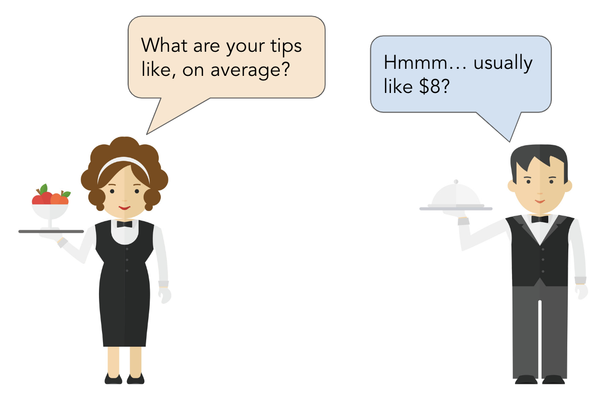
Example: Restaurant tips 🧑🍳
About the data
What features does the dataset contain? Is this likely a recent dataset, or an older one?
# The dataset is built into plotly!
tips = px.data.tips()
tips
| total_bill | tip | sex | smoker | day | time | size | |
|---|---|---|---|---|---|---|---|
| 0 | 16.99 | 1.01 | Female | No | Sun | Dinner | 2 |
| 1 | 10.34 | 1.66 | Male | No | Sun | Dinner | 3 |
| 2 | 21.01 | 3.50 | Male | No | Sun | Dinner | 3 |
| ... | ... | ... | ... | ... | ... | ... | ... |
| 241 | 22.67 | 2.00 | Male | Yes | Sat | Dinner | 2 |
| 242 | 17.82 | 1.75 | Male | No | Sat | Dinner | 2 |
| 243 | 18.78 | 3.00 | Female | No | Thur | Dinner | 2 |
244 rows × 7 columns
Predicting tips
- Goal: Given various information about a table at a restaurant, we want to predict the tip that a server will earn.
- Why might a server be interested in doing this?
- To determine which tables are likely to tip the most (inference).
- To predict earnings over the next month (prediction).
Exploratory data analysis
- The most natural feature to look at first is total bills.
- As such, we should explore the relationship between total bills and tips. Moving forward:
- $x$: Total bills.
- $y$: Tips.
fig = tips.plot(kind='scatter', x='total_bill', y='tip', title='Tip vs. Total Bill')
fig.update_layout(xaxis_title='Total Bill', yaxis_title='Tip')
Model #1: Constant
- Let's start simple, by ignoring all features. Suppose our model assumes every tip is given by a constant dollar amount:
$$\text{tip} = h^{\text{true}}$$
- Model: There is a single tip amount $h^{\text{true}}$ that all customers pay.
- Correct? No!
- Useful? Perhaps. An estimate of $h^{\text{true}}$, denoted by $h^*$, can allow us to predict future tips.
Estimating $h^{\text{true}}$
- The true parameter $h^{\text{true}}$ is determined by the universe. We'll never get to see it, so we need to estimate it.
- There are several ways we could estimate $h^{\text{true}}$. For instance, we could use domain knowledge: for instance, assume that everyone clicks the $1 tip option when buying coffee.
- But, perhaps, we should look at the tips that we've already seen in our dataset to estimate $h^{\text{true}}$.
Looking at the data
Our estimate for $h^{\text{true}}$ should be a good summary statistic of the distribution of tips.
fig = tips.plot(kind='hist', x='tip', title='Distribution of Tip', nbins=20)
fig.update_layout(xaxis_title='Tip', yaxis_title='Frequency')
Empirical risk minimization
- In DSC 40A, we established a framework for estimating model parameters:
- Choose a loss function, which measures how "good" a single prediction is.
- Minimize empirical risk, to find the best estimate for the dataset that we have.
- Depending on which loss function we choose, we will end up with different $h^*$ (which are estimates of $h^{\text{true}})$.
- If we choose squared loss, then our empirical risk is mean squared error:
$$\text{MSE} = \frac{1}{n} \sum_{i = 1}^n ( y_i - h )^2 \overset{\text{calculus}}\implies h^* = \text{mean}(y)$$
- If we choose absolute loss, then our empirical risk is mean absolute error:
$$\text{MAE} = \frac{1}{n} \sum_{i = 1}^n | y_i - h | \overset{\text{algebra}}\implies h^* = \text{median}(y)$$
The mean tip
Let's suppose we choose squared loss, meaning that $h^* = \text{mean}(y)$.
mean_tip = tips['tip'].mean()
mean_tip
np.float64(2.99827868852459)
$h^* = 2.998$ is our fit model – it was fit to our training data (the data we have available to learn from).
Let's visualize this prediction.
fig = px.scatter(tips, x='total_bill', y='tip')
fig.add_hline(mean_tip, line_width=3, line_color='orange', opacity=1)
fig.update_layout(title='Tip vs. Total Bill',
xaxis_title='Total Bill', yaxis_title='Tip')
Note that to make predictions, this model ignores total bill (and all other features), and predicts the same tip for all tables.
The quality of predictions
- Question: How can we quantify how good this constant prediction is at predicting tips in our training data – that is, the data we used to fit the model?
- One answer: use the mean squared error. If $y_i$ represents the $i$th actual value and $H(x_i)$ represents the $i$th predicted value, then:
$$\text{MSE} = \frac{1}{n} \sum_{i = 1}^n \big( y_i - H(x_i) \big)^2$$
np.mean((tips['tip'] - mean_tip) ** 2)
np.float64(1.9066085124966412)
# The same! A fact from 40A.
np.var(tips['tip'])
np.float64(1.9066085124966412)
- Issue: The units of MSE are "dollars squared", which are a little hard to interpret.
Root mean squared error
- Often, to measure the quality of a regression model's predictions, we will use the root mean squared error (RMSE):
$$\text{RMSE} = \sqrt{\frac{1}{n} \sum_{i = 1}^n \big( y_i - H(x_i) \big)^2}$$
- The units of the RMSE are the same as the units of the original $y$ values – dollars, in this case.
- Important: Minimizing MSE is the same as minimizing RMSE; the constant tip $h^*$ that minimizes MSE is the same $h^*$ that minimizes RMSE. (Why?)
Computing and storing the RMSE
Since we'll compute the RMSE for our future models too, we'll define a function that can compute it for us.
def rmse(actual, pred):
return np.sqrt(np.mean((actual - pred) ** 2))
Let's compute the RMSE of our constant tip's predictions, and store it in a dictionary that we can refer to later on.
rmse(tips['tip'], mean_tip)
np.float64(1.3807999538298954)
rmse_dict = {}
rmse_dict['constant tip amount'] = rmse(tips['tip'], mean_tip)
rmse_dict
{'constant tip amount': np.float64(1.3807999538298954)}
Key idea: Since the mean minimizes RMSE for the constant model, it is impossible to change the mean_tip argument above to another number and yield a lower RMSE.
Model #2: Simple linear regression using total bill
- We haven't yet used any of the features in the dataset. The first natural feature to look at is
'total_bill'.
tips.head()
| total_bill | tip | sex | smoker | day | time | size | |
|---|---|---|---|---|---|---|---|
| 0 | 16.99 | 1.01 | Female | No | Sun | Dinner | 2 |
| 1 | 10.34 | 1.66 | Male | No | Sun | Dinner | 3 |
| 2 | 21.01 | 3.50 | Male | No | Sun | Dinner | 3 |
| 3 | 23.68 | 3.31 | Male | No | Sun | Dinner | 2 |
| 4 | 24.59 | 3.61 | Female | No | Sun | Dinner | 4 |
- We can fit a simple linear model to predict tips as a function of total bills:
$$\text{predicted tip} = w_0 + w_1 \cdot \text{total bill}$$
- This is a reasonable thing to do, because total bills and tips appeared to be linearly associated when we visualized them on a scatter plot a few slides ago.
Recap: Simple linear regression
A simple linear regression model is a linear model with a single feature, as we have here. For any total bill $x_i$, the predicted tip $H(x_i)$ is given by
$$H(x_i) = w_0 + w_1x_i$$
- Question: How do we determine which intercept, $w_0$, and slope, $w_1$, to use?
- One answer: Pick the $w_0$ and $w_1$ that minimize mean squared error. If $x_i$ and $y_i$ correspond to the $i$th total bill and tip, respectively, then:
$$\begin{align*}\text{MSE} &= \frac{1}{n} \sum_{i = 1}^n \big( y_i - H(x_i) \big)^2 \\ &= \frac{1}{n} \sum_{i = 1}^n \big( y_i - w_0 - w_1x_i \big)^2\end{align*}$$
- Key idea: The lower the MSE on our training data is, the "better" the model fits the training data.
- Lower MSE = better predictions.
- But lower MSE ≠ more reflective of reality!
Empirical risk minimization, by hand
$$\begin{align*}\text{MSE} &= \frac{1}{n} \sum_{i = 1}^n \big( y_i - w_0 - w_1x_i \big)^2\end{align*}$$
- In DSC 40A, you found the formulas for the best intercept, $w_0^*$, and the best slope, $w_1^*$, through calculus.
- The resulting line, $H(x_i) = w_0^* + w_1^* x_i$, is called the line of best fit, or the regression line.
- Specifically, if $r$ is the correlation coefficient, $\sigma_x$ and $\sigma_y$ are the standard deviations of $x$ and $y$, and $\bar{x}$ and $\bar{y}$ are the means of $x$ and $y$, then:
$$w_1^* = r \cdot \frac{\sigma_y}{\sigma_x}$$
$$w_0^* = \bar{y} - w_1^* \bar{x}$$
Regression in sklearn
sklearn

sklearn(scikit-learn) implements many common steps in the feature and model creation pipeline.- It is widely used throughout industry and academia.
- It interfaces with
numpyarrays, and to an extent,pandasDataFrames.
- Huge benefit: the documentation online is excellent.
The LinearRegression class
sklearncomes with several subpackages, includinglinear_modelandtree, each of which contains several classes of models.
- We'll start with the
LinearRegressionclass fromlinear_model.
from sklearn.linear_model import LinearRegression
- Important: From the documentation, we have:
LinearRegression fits a linear model with coefficients w = (w1, …, wp) to minimize the residual sum of squares between the observed targets in the dataset, and the targets predicted by the linear approximation.
In other words, **`LinearRegression` minimizes mean squared error by default**! (Per the documentation, it also includes an intercept term by default.)LinearRegression?
Init signature: LinearRegression( *, fit_intercept=True, copy_X=True, n_jobs=None, positive=False, ) Docstring: Ordinary least squares Linear Regression. LinearRegression fits a linear model with coefficients w = (w1, ..., wp) to minimize the residual sum of squares between the observed targets in the dataset, and the targets predicted by the linear approximation. Parameters ---------- fit_intercept : bool, default=True Whether to calculate the intercept for this model. If set to False, no intercept will be used in calculations (i.e. data is expected to be centered). copy_X : bool, default=True If True, X will be copied; else, it may be overwritten. n_jobs : int, default=None The number of jobs to use for the computation. This will only provide speedup in case of sufficiently large problems, that is if firstly `n_targets > 1` and secondly `X` is sparse or if `positive` is set to `True`. ``None`` means 1 unless in a :obj:`joblib.parallel_backend` context. ``-1`` means using all processors. See :term:`Glossary <n_jobs>` for more details. positive : bool, default=False When set to ``True``, forces the coefficients to be positive. This option is only supported for dense arrays. .. versionadded:: 0.24 Attributes ---------- coef_ : array of shape (n_features, ) or (n_targets, n_features) Estimated coefficients for the linear regression problem. If multiple targets are passed during the fit (y 2D), this is a 2D array of shape (n_targets, n_features), while if only one target is passed, this is a 1D array of length n_features. rank_ : int Rank of matrix `X`. Only available when `X` is dense. singular_ : array of shape (min(X, y),) Singular values of `X`. Only available when `X` is dense. intercept_ : float or array of shape (n_targets,) Independent term in the linear model. Set to 0.0 if `fit_intercept = False`. n_features_in_ : int Number of features seen during :term:`fit`. .. versionadded:: 0.24 feature_names_in_ : ndarray of shape (`n_features_in_`,) Names of features seen during :term:`fit`. Defined only when `X` has feature names that are all strings. .. versionadded:: 1.0 See Also -------- Ridge : Ridge regression addresses some of the problems of Ordinary Least Squares by imposing a penalty on the size of the coefficients with l2 regularization. Lasso : The Lasso is a linear model that estimates sparse coefficients with l1 regularization. ElasticNet : Elastic-Net is a linear regression model trained with both l1 and l2 -norm regularization of the coefficients. Notes ----- From the implementation point of view, this is just plain Ordinary Least Squares (scipy.linalg.lstsq) or Non Negative Least Squares (scipy.optimize.nnls) wrapped as a predictor object. Examples -------- >>> import numpy as np >>> from sklearn.linear_model import LinearRegression >>> X = np.array([[1, 1], [1, 2], [2, 2], [2, 3]]) >>> # y = 1 * x_0 + 2 * x_1 + 3 >>> y = np.dot(X, np.array([1, 2])) + 3 >>> reg = LinearRegression().fit(X, y) >>> reg.score(X, y) 1.0 >>> reg.coef_ array([1., 2.]) >>> reg.intercept_ np.float64(3.0...) >>> reg.predict(np.array([[3, 5]])) array([16.]) File: ~/miniforge3/envs/dsc80/lib/python3.12/site-packages/sklearn/linear_model/_base.py Type: ABCMeta Subclasses:
Fitting a simple linear model
First, we must instantiate a LinearRegression object and fit it. By calling fit, we are saying "minimize mean squared error on this dataset and find $w^*$."
model = LinearRegression()
# Note that there are two arguments to fit – X and y!
# (It is not necessary to write X= and y=)
model.fit(X=tips[['total_bill']], y=tips['tip'])
LinearRegression()In a Jupyter environment, please rerun this cell to show the HTML representation or trust the notebook.
On GitHub, the HTML representation is unable to render, please try loading this page with nbviewer.org.
LinearRegression()
After fitting, we can access $w^*$ – that is, the best slope and intercept.
model.intercept_, model.coef_[0]
(np.float64(0.920269613554674), np.float64(0.10502451738435332))
These coefficients tell us that the "best way" (according to squared loss) to make tip predictions using a linear model is using:
$$\text{predicted tip} = 0.92 + 0.105 \cdot \text{total bill}$$
This model predicts that people tip by:
- Tipping a constant 92 cents.
- Tipping 10.5% for every dollar spent.
This is the best "linear" pattern in the dataset – it doesn't mean this is actually how people tip!
Let's visualize this model, along with our previous model.
line_pts = pd.DataFrame({'total_bill': [0, 60]})
fig = px.scatter(tips, x='total_bill', y='tip')
fig.add_trace(go.Scatter(
x=line_pts['total_bill'],
y=[mean_tip, mean_tip],
mode='lines',
name='Constant Model (Mean Tip)'
))
fig.add_trace(go.Scatter(
x=line_pts['total_bill'],
y=model.predict(line_pts),
mode='lines',
name='Linear Model: Total Bill Only'
))
fig.update_layout(title='Tip vs. Total Bill',
xaxis_title='Total Bill',
yaxis_title='Tip')
Visually, our linear model seems to be a better fit for our dataset than our constant model.
Can we quantify whether or not it is better?
Making predictions
Fit LinearRegression objects also have a predict method, which can be used to predict tips for any total bill, new or old.
model.predict([[15]])
/Users/sam/miniforge3/envs/dsc80/lib/python3.12/site-packages/sklearn/base.py:493: UserWarning: X does not have valid feature names, but LinearRegression was fitted with feature names
array([2.5])
# Since we trained on a DataFrame, the input to model.predict should also
# be a DataFrame. To avoid having to do this, we can use .to_numpy()
# when specifying X= and y=.
test_points = pd.DataFrame({'total_bill': [15, 4, 100]})
model.predict(test_points)
array([ 2.5 , 1.34, 11.42])
Comparing models
If we want to compute the RMSE of our model on the training data, we need to find its predictions on every row in the training data, tips.
all_preds = model.predict(tips[['total_bill']])
rmse_dict['one feature: total bill'] = rmse(tips['tip'], all_preds)
rmse_dict
{'constant tip amount': np.float64(1.3807999538298954),
'one feature: total bill': np.float64(1.0178504025697377)}
- The RMSE of our simple linear model is lower than that of our constant model, which means it does a better job at predicting tips in our training data than our constant model.
- Theory tells us it's impossible for the RMSE on the training data to increase as we add more features to the same model. However, the RMSE may increase on unseen data by adding more features; we'll discuss this idea more soon.
💡 Pro-Tip: Making a DF just to display
Sometimes it's nice to put your values into a dataframe just to make them display nicely:
rmse_dict
{'constant tip amount': np.float64(1.3807999538298954),
'one feature: total bill': np.float64(1.0178504025697377)}
pd.DataFrame({'rmse': rmse_dict.values()}, index=rmse_dict.keys())
| rmse | |
|---|---|
| constant tip amount | 1.38 |
| one feature: total bill | 1.02 |
Model #3: Multiple linear regression using total bill and table size
- There are still many features in
tipswe haven't touched:
tips.head()
| total_bill | tip | sex | smoker | day | time | size | |
|---|---|---|---|---|---|---|---|
| 0 | 16.99 | 1.01 | Female | No | Sun | Dinner | 2 |
| 1 | 10.34 | 1.66 | Male | No | Sun | Dinner | 3 |
| 2 | 21.01 | 3.50 | Male | No | Sun | Dinner | 3 |
| 3 | 23.68 | 3.31 | Male | No | Sun | Dinner | 2 |
| 4 | 24.59 | 3.61 | Female | No | Sun | Dinner | 4 |
- Let's try using another feature – table size. Such a model would predict tips using:
$$\text{predicted tip} = w_0 + w_1 \cdot \text{total bill} + w_2 \cdot \text{table size}$$
Multiple linear regression
To find the optimal parameters $w^*$, we will again use sklearn's LinearRegression class. The code is not all that different!
model_two = LinearRegression()
model_two.fit(X=tips[['total_bill', 'size']], y=tips['tip'])
LinearRegression()In a Jupyter environment, please rerun this cell to show the HTML representation or trust the notebook.
On GitHub, the HTML representation is unable to render, please try loading this page with nbviewer.org.
LinearRegression()
model_two.intercept_, model_two.coef_
(np.float64(0.6689447408125035), array([0.09, 0.19]))
test_pts = pd.DataFrame({'total_bill': [25], 'size': [4]})
model_two.predict(test_pts)
array([3.76])
What does this model look like?
Plane of best fit ✈️
Here, we must draw a 3D scatter plot and plane, with one axis for total bill, one axis for table size, and one axis for tip. The code below does this.
XX, YY = np.mgrid[0:50:2, 0:8:1]
Z = model_two.intercept_ + model_two.coef_[0] * XX + model_two.coef_[1] * YY
plane = go.Surface(x=XX, y=YY, z=Z, colorscale='Oranges')
fig = go.Figure(data=[plane])
fig.add_trace(go.Scatter3d(x=tips['total_bill'],
y=tips['size'],
z=tips['tip'], mode='markers',
marker={'color': '#656DF1', 'size': 5}))
fig.update_layout(scene=dict(xaxis_title='Total Bill',
yaxis_title='Table Size',
zaxis_title='Tip'),
title='Tip vs. Total Bill and Table Size',
width=500, height=500)
Comparing models, again
How does our two-feature linear model stack up to our single feature linear model and our constant model?
rmse_dict['two features'] = rmse(
tips['tip'], model_two.predict(tips[['total_bill', 'size']])
)
pd.DataFrame({'rmse': rmse_dict.values()}, index=rmse_dict.keys())
| rmse | |
|---|---|
| constant tip amount | 1.38 |
| one feature: total bill | 1.02 |
| two features | 1.01 |
- The RMSE of our two-feature model is the lowest of the three models we've looked at so far, but not by much. We didn't gain much by adding table size to our linear model.
- It's also not clear whether table sizes are practically useful in predicting tips.
- We already have the total amount the table spent; why do we need to know how many people were there?
Residual plots
- From DSC 10: one important technique for diagnosing model fit is the residual plot.
- The $i$th residual is $ y_i - H(x_i) $.
- A residual plot has
- predicted values $H(x)$ on the $x$-axis, and
- residuals $ y - H(x) $ on the $y$-axis.
# Let's start with the single-variable model:
with_resid = tips.assign(**{
'Predicted Tip': model.predict(tips[['total_bill']]),
'Residual': tips['tip'] - model.predict(tips[['total_bill']]),
})
fig = px.scatter(with_resid, x='Predicted Tip', y='Residual')
fig.add_hline(0, line_width=2, opacity=1).update_layout(title='Residual Plot (Simple Linear Model)')
- If all assumptions about linear regression hold, then residual plot should look randomly scattered around the horizontal line $y = 0$.
- Here, we see that the model makes bigger mistakes for larger predicted values. But overall, there's no apparent trend, so a linear model seems appropriate.
# What about the two-variable model?
with_resid = tips.assign(**{
'Predicted Tip': model_two.predict(tips[['total_bill', 'size']]),
'Residual': tips['tip'] - model_two.predict(tips[['total_bill', 'size']]),
})
fig = px.scatter(with_resid, x='Predicted Tip', y='Residual')
fig.add_hline(0, line_width=2, opacity=1).update_layout(title='Residual Plot (Multiple Regression)')
Looks about the same as the previous plot!
Question 🤔 (Answer at dsc80.com/q)
Code: resids
Consider the following dataframe grades that has a midterm and final column.
Ask ChatGPT to make two plots using plotly:
- A regular residual plot.
- A residual plot that accidentally puts the original
finalon the x-axis instead of the predicted values.
What do you notice?
grades = pd.read_csv('data/gradesW4315.csv')[['midterm', 'final']]
grades
| midterm | final | |
|---|---|---|
| 0 | 80 | 103 |
| 1 | 53 | 79 |
| 2 | 91 | 122 |
| ... | ... | ... |
| 49 | 77 | 98 |
| 50 | 70 | 134 |
| 51 | 75 | 99 |
52 rows × 2 columns
Summary, next time
Summary
- We built three models:
- A constant model: $\text{predicted tip} = h^*$.
- A simple linear regression model: $\text{predicted tip} = w_0^* + w_1^* \cdot \text{total bill}$.
- A multiple linear regression model: $\text{predicted tip} = w_0^* + w_1^* \cdot \text{total bill} + w_2^* \cdot \text{table size}$.
- As we added more features, our RMSEs decreased.
- This was guaranteed to happen, since we were only looking at our training data.
- It is not clear that the final linear model is actually "better"; it doesn't seem to reflect reality better than the previous models.
LinearRegression summary
| Property | Example | Description |
|---|---|---|
| Initialize model parameters | lr = LinearRegression() |
Create (empty) linear regression model |
| Fit the model to the data | lr.fit(X, y) |
Determines regression coefficients |
| Use model for prediction | lr.predict(X_new) |
Uses regression line to make predictions |
| Evaluate the model | lr.score(X, y) |
Calculates the $R^2$ of the LR model |
| Access model attributes | lr.coef_, lr.intercept_ |
Accesses the regression coefficients and intercept |
Next time
tips.head()
| total_bill | tip | sex | smoker | day | time | size | |
|---|---|---|---|---|---|---|---|
| 0 | 16.99 | 1.01 | Female | No | Sun | Dinner | 2 |
| 1 | 10.34 | 1.66 | Male | No | Sun | Dinner | 3 |
| 2 | 21.01 | 3.50 | Male | No | Sun | Dinner | 3 |
| 3 | 23.68 | 3.31 | Male | No | Sun | Dinner | 2 |
| 4 | 24.59 | 3.61 | Female | No | Sun | Dinner | 4 |
So far, in our journey to predict
'tip', we've only used the existing numerical features in our dataset,'total_bill'and'size'.There's a lot of information in tips that we didn't use –
'sex','smoker','day', and'time', for example. We can't use these features in their current form, because they're non-numeric.How do we use categorical features in a regression model?