from dsc80_utils import *

Lecture 18 – Classifier Evaluation, Model Fairness

DSC 80, Fall 2024

Announcements 📣

• Lab 9 deadline moved to Monday Dec 2 since Thanksgiving is this week.

• Guest lecture on Thursday Dec 5, 1:30pm-3pm in the HDSI MPR: Dr. Mohammad Ramezanali, an AI lead from Salesforce, will be talking about LLMs and how he uses them in industry.

  • No regular lecture on Dec 5.
  • If you attend the guest lecture, you will get lecture attendance credit and 1% extra credit on your final exam grade.
  • If you can't make it, we'll record the talk and you can get attendance + extra credit by making a post on Ed with a few paragraphs about the talk (details to come).

• The Final Project is due on Friday Dec 6.

  • No slip days allowed!

• The Final Exam is on Saturday, Dec 7 from 11:30am-2:30pm in PODEM 1A18 and 1A19.

  • Practice by working through old exams at practice.dsc80.com.
  • You can bring two double-sided notes sheets
  • Will post on Ed for more details.

• Thursday's class will start with career advice, then rest of time is exam review!

Final Exam 📝

• Saturday, Dec 7 from 11:30am-2:30pm in PODEM 1A18 and 1A19.
  • Will write the exam to take about 2 hours, so you'll have a lot of time to double check your work.
• Two 8.5"x11" cheat sheets allowed of your own creation (handwritten on tablet, then printed is okay.)
• Covers every lecture, lab, and project.
• Similar format to the midterm: mix of fill-in-the-blank, multiple choice, and free response.
  • I use pandas fill-in-the-blank questions to test your ability to read and write code, not just write code from scratch, which is why they can feel tricker.
• Questions on final about pre-Midterm material will be marked as "M". Your Midterm grade will be the higher of your (z-score adjusted) grades on the Midterm and the questions marked as "M" on the final.

Agenda 📆

• Classifier evaluation.
• Logistic regression.
• Model fairness.

Aside: MLU Explain is a great resource with visual explanations of many of our recent topics (cross-validation, random forests, precision and recall, etc.).

Random Forests

diabetes = pd.read_csv(Path('data') / 'diabetes.csv')
display_df(diabetes, cols=9)

	Pregnancies	Glucose	BloodPressure	SkinThickness	Insulin	BMI	DiabetesPedigreeFunction	Age	Outcome
0	6	148	72	35	0	33.6	0.63	50	1
1	1	85	66	29	0	26.6	0.35	31	0
2	8	183	64	0	0	23.3	0.67	32	1
...	...	...	...	...	...	...	...	...	...
765	5	121	72	23	112	26.2	0.24	30	0
766	1	126	60	0	0	30.1	0.35	47	1
767	1	93	70	31	0	30.4	0.32	23	0

768 rows × 9 columns

from sklearn.model_selection import train_test_split
X_train, X_test, y_train, y_test = (
    train_test_split(diabetes[['Glucose', 'BMI']], diabetes['Outcome'], random_state=1)
)

fig = (
    X_train.assign(Outcome=y_train.astype(str))
            .plot(kind='scatter', x='Glucose', y='BMI', color='Outcome', 
                  color_discrete_map={'0': 'orange', '1': 'blue'},
                  title='Relationship between Glucose, BMI, and Diabetes')
)
fig

Random Forests

Main idea:

Train a bunch of decision trees, then have them vote on a prediction!

• Problem: If you use the same training data, you will always get the same tree.
• Solution: Introduce randomness into training procedure to get different trees.

Idea 1: Bootstrap the training data

• We can bootstrap the training data $T$ times, then train one tree on each resample.
• Also known as bagging (Bootstrap AGgregating). In general, combining different predictors together is a useful technique called ensemble learning.
• For decision trees though, doesn't make trees different enough from each other (e.g. if you have one really strong predictor, it'll always be the first split).

Idea 2: Only use a subset of features

• At each split, take a random subset of $ m $ features instead of choosing from all $ d $ of them.

• Rule of thumb: $ m \approx \sqrt d $ seems to work well.

• Key idea: For ensemble learning, you want the individual predictors to have low bias, high variance, and be uncorrelated with each other. That way, when you average them together, you have low bias AND low variance.

• Random forest algorithm: Fit $ T $ trees by using bagging and a random subset of features at each split. Predict by taking a vote from the $ T $ trees.

Question 🤔 (Answer at dsc80.com/q)

Code: bvm

How will increasing $ m $ affect the bias / variance of each decision tree?

Example

# Let's use more features for prediction
from sklearn.model_selection import train_test_split
X_train, X_test, y_train, y_test = (
    train_test_split(diabetes.drop(columns=['Outcome']), diabetes['Outcome'], random_state=1)
)

from sklearn.ensemble import RandomForestClassifier

clf = RandomForestClassifier()
clf.fit(X_train, y_train)
clf.score(X_train, y_train)

1.0

clf.score(X_test, y_test)

0.8020833333333334

Compared to our previous best decision tree with depth 4:

from sklearn.tree import DecisionTreeClassifier
dt = DecisionTreeClassifier(max_depth=4, criterion='entropy')
dt.fit(X_train, y_train)
dt.score(X_train, y_train)

0.7829861111111112

dt.score(X_test, y_test)

0.7395833333333334

Example: Modeling using text features

Example: Fake news

We have a dataset containing news articles and labels for whether the article was deemed "fake" or "real". Credit to https://github.com/KaiDMML/FakeNewsNet.

news = pd.read_csv('data/fake_news_training.csv')
news

	baseurl	content	label
0	twitter.com	\njavascript is not available.\n\nwe’ve detect...	real
1	whitehouse.gov	remarks by the president at campaign event -- ...	real
2	web.archive.org	the committee on energy and commerce\nbarton: ...	real
...	...	...	...
658	politico.com	full text: jeff flake on trump speech transcri...	fake
659	pol.moveon.org	moveon.org political action: 10 things to know...	real
660	uspostman.com	uspostman.com is for sale\nyes, you can transf...	fake

661 rows × 3 columns

Goal: Use an article's content to predict its label.

news['label'].value_counts(normalize=True)

label
real    0.55
fake    0.45
Name: proportion, dtype: float64

Question: What is the worst possible accuracy we should expect from a classifier, given the above distribution?

Aside: CountVectorizer

Entries in the 'content' column are not currently quantitative! We can use the bag of words encoding to create quantitative features out of each 'content'.

Instead of performing a bag of words encoding manually as we did before, we can rely on sklearn's CountVectorizer. (There is also a TfidfVectorizer.)

from sklearn.feature_extraction.text import CountVectorizer

example_corp = ['hey hey hey my name is billy', 
                'hey billy how is your dog billy']

count_vec = CountVectorizer()
count_vec.fit(example_corp)

CountVectorizer()

In a Jupyter environment, please rerun this cell to show the HTML representation or trust the notebook.
On GitHub, the HTML representation is unable to render, please try loading this page with nbviewer.org.

count_vec learned a vocabulary from the corpus we fit it on.

count_vec.vocabulary_

{'hey': 2,
 'my': 5,
 'name': 6,
 'is': 4,
 'billy': 0,
 'how': 3,
 'your': 7,
 'dog': 1}

count_vec.transform(example_corp).toarray()

array([[1, 0, 3, 0, 1, 1, 1, 0],
       [2, 1, 1, 1, 1, 0, 0, 1]])

Note that the values in count_vec.vocabulary_ correspond to the positions of the columns in count_vec.transform(example_corp).toarray(), i.e. 'billy' is the first column and 'your' is the last column.

example_corp

['hey hey hey my name is billy', 'hey billy how is your dog billy']

pd.DataFrame(count_vec.transform(example_corp).toarray(),
             columns=pd.Series(count_vec.vocabulary_).sort_values().index)

	billy	dog	hey	how	is	my	name	your
0	1	0	3	0	1	1	1	0
1	2	1	1	1	1	0	0	1

Creating an initial Pipeline

Let's build a Pipeline that takes in summaries and overall ratings and:

• Uses CountVectorizer to quantitatively encode summaries.

• Fits a RandomForestClassifier to the data.

But first, a train-test split (like always).

from sklearn.model_selection import train_test_split
from sklearn.pipeline import Pipeline
from sklearn.ensemble import RandomForestClassifier

X = news['content']
y = news['label']
X_train, X_test, y_train, y_test = train_test_split(X, y)

To start, we'll create a random forest with 100 trees (n_estimators) each of which has a maximum depth of 3 (max_depth).

pl = Pipeline([
    ('cv', CountVectorizer()), 
    ('clf', RandomForestClassifier(
        max_depth=3,
        n_estimators=100, # Uses 100 separate decision trees!
        random_state=42,
    )) 
])

pl.fit(X_train, y_train)

Pipeline(steps=[('cv', CountVectorizer()),
                ('clf', RandomForestClassifier(max_depth=3, random_state=42))])

In a Jupyter environment, please rerun this cell to show the HTML representation or trust the notebook.
On GitHub, the HTML representation is unable to render, please try loading this page with nbviewer.org.

# Training accuracy.
pl.score(X_train, y_train)

0.7393939393939394

# Testing accuracy.
pl.score(X_test, y_test)

0.7108433734939759

The accuracy of our random forest is just under 73%, on the test set. How much better does it do compared to a classifier that predicts "real" every time?

y_train.value_counts(normalize=True)

label
real    0.54
fake    0.46
Name: proportion, dtype: float64

# Distribution of predicted ys in the training set:

# stops scientific notation for pandas
pd.set_option('display.float_format', '{:.3f}'.format)
pd.Series(pl.predict(X_train)).value_counts(normalize=True)

fake   0.689
real   0.311
Name: proportion, dtype: float64

len(pl.named_steps['cv'].vocabulary_) # Lots of features!

23527

Choosing tree depth via GridSearchCV

We arbitrarily chose max_depth=3 before, but it seems like that isn't working well. Let's perform a grid search to find the max_depth with the best generalization performance.

# Note that we've used the key clf__max_depth, not max_depth
# because max_depth is a hyperparameter of clf, not of pl.

hyperparameters = {
    'clf__max_depth': np.arange(2, 200, 20)
}

Note that while pl has already been fit, we can still give it to GridSearchCV, which will repeatedly re-fit it during cross-validation.

%%time

# Takes a few seconds to run – how many trees are being trained?
from sklearn.model_selection import GridSearchCV
grids = GridSearchCV(
    pl,
    n_jobs=-1, # Use multiple processors to parallelize
    param_grid=hyperparameters,
    return_train_score=True
)
grids.fit(X_train, y_train)

CPU times: user 1.24 s, sys: 313 ms, total: 1.55 s
Wall time: 6.12 s

GridSearchCV(estimator=Pipeline(steps=[('cv', CountVectorizer()),
                                       ('clf',
                                        RandomForestClassifier(max_depth=3,
                                                               random_state=42))]),
             n_jobs=-1,
             param_grid={'clf__max_depth': array([  2,  22,  42,  62,  82, 102, 122, 142, 162, 182])},
             return_train_score=True)

In a Jupyter environment, please rerun this cell to show the HTML representation or trust the notebook.
On GitHub, the HTML representation is unable to render, please try loading this page with nbviewer.org.

grids.best_params_

{'clf__max_depth': np.int64(42)}

Recall, fit GridSearchCV objects are estimators on their own as well. This means we can compute the training and testing accuracies of the "best" random forest directly:

# Training accuracy.
grids.score(X_train, y_train)

0.9959595959595959

# Testing accuracy.
grids.score(X_test, y_test)

0.8373493975903614

~10% better test set error!

Training and validation accuracy vs. depth

Below, we plot how training and validation accuracy varied with tree depth. Note that the $y$-axis here is accuracy, and that larger accuracies are better (unlike with RMSE, where smaller was better).

index = grids.param_grid['clf__max_depth']
train = grids.cv_results_['mean_train_score']
valid = grids.cv_results_['mean_test_score']

pd.DataFrame({'train': train, 'valid': valid}, index=index).plot().update_layout(
    xaxis_title='max_depth', yaxis_title='Accuracy'
)

Question 🤔 (Answer at dsc80.com/q)

Code: fa23102

(Fa23 Final Q10.2)

Suppose we write the following code:

hyperparameters = {
    'n_estimators': [10, 100, 1000], # number of trees per forest
    'max_depth': [None, 100, 10]     # max depth of each tree
}
grids = GridSearchCV(
    RandomForestClassifier(), param_grid=hyperparameters,
    cv=3, # 3-fold cross-validation
)
grids.fit(X_train, y_train)

Answer the following questions with a single number.

1. How many random forests are fit in total?
2. How many decision trees are fit in total?
3. How many times in total is the first point in X_train used to train a decision tree?

Classifier Evaluation

Accuracy isn't everything!

$$ \text{accuracy} = \frac{\text{\# data points classified correctly}}{\text{\# data points}} $$

• Accuracy is defined as the proportion of predictions that are correct.

• It weighs all correct predictions the same, and weighs all incorrect predictions the same.

• But some incorrect predictions may be worse than others!

  • Example: Suppose you take a COVID test 🦠. Which is worse:
    • The test saying you have COVID, when you really don't, or
    • The test saying you don't have COVID, when you really do?

The Boy Who Cried Wolf 👦😭🐺

(source)

A shepherd boy gets bored tending the town's flock. To have some fun, he cries out, "Wolf!" even though no wolf is in sight. The villagers run to protect the flock, but then get really mad when they realize the boy was playing a joke on them.

Repeat the previous paragraph many, many times.

One night, the shepherd boy sees a real wolf approaching the flock and calls out, "Wolf!" The villagers refuse to be fooled again and stay in their houses. The hungry wolf turns the flock into lamb chops. The town goes hungry. Panic ensues.

The wolf classifier

• Predictor: Shepherd boy.
• Positive prediction: "There is a wolf."
• Negative prediction: "There is no wolf."

Some questions to think about:

• What is an example of an incorrect, positive prediction?

• Was there a correct, negative prediction?

• There are four possibilities. What are the consequences of each?
  • (predict yes, predict no) x (actually yes, actually no).

The wolf classifier

Below, we present a confusion matrix, which summarizes the four possible outcomes of the wolf classifier.

Outcomes in binary classification

When performing binary classification, there are four possible outcomes.

(Note: A "positive prediction" is a prediction of 1, and a "negative prediction" is a prediction of 0.)

Outcome of Prediction	Definition	True Class
True positive (TP) ✅	The predictor correctly predicts the positive class.	P
False negative (FN) ❌	The predictor incorrectly predicts the negative class.	P
True negative (TN) ✅	The predictor correctly predicts the negative class.	N
False positive (FP) ❌	The predictor incorrectly predicts the positive class.	N

⬇️

	Predicted Negative	Predicted Positive
Actually Negative	TN ✅	FP ❌
Actually Positive	FN ❌	TP ✅

The confusion matrix above is organized the same way that sklearn's confusion matrices are (but differently than in the wolf example).

Note that in the four acronyms – TP, FN, TN, FP – the first letter is whether the prediction is correct, and the second letter is what the prediction is.

Example: COVID testing 🦠

• UCSD Health administers hundreds of COVID tests a day. The tests are not fully accurate.

• Each test comes back either

  • positive, indicating that the individual has COVID, or
  • negative, indicating that the individual does not have COVID.

• Question: What is a TP in this scenario? FP? TN? FN?

• TP: The test predicted that the individual has COVID, and they do ✅.

• FP: The test predicted that the individual has COVID, but they don't ❌.

• TN: The test predicted that the individual doesn't have COVID, and they don't ✅.

• FN: The test predicted that the individual doesn't have COVID, but they do ❌.

Accuracy of COVID tests

The results of 100 UCSD Health COVID tests are given below.

	Predicted Negative	Predicted Positive
Actually Negative	TN = 90 ✅	FP = 1 ❌
Actually Positive	FN = 8 ❌	TP = 1 ✅

UCSD Health test results

🤔 Question: What is the accuracy of the test?

🙋 Answer: $$\text{accuracy} = \frac{TP + TN}{TP + FP + FN + TN} = \frac{1 + 90}{100} = 0.91$$

• Followup: At first, the test seems good. But, suppose we build a classifier that predicts that nobody has COVID. What would its accuracy be?

• Answer to followup: Also 0.91! There is severe class imbalance in the dataset, meaning that most of the data points are in the same class (no COVID). Accuracy doesn't tell the full story.

Recall

	Predicted Negative	Predicted Positive
Actually Negative	TN = 90 ✅	FP = 1 ❌
Actually Positive	FN = 8 ❌	TP = 1 ✅

UCSD Health test results

🤔 Question: What proportion of individuals who actually have COVID did the test identify?

🙋 Answer: $\frac{1}{1 + 8} = \frac{1}{9} \approx 0.11$

More generally, the recall of a binary classifier is the proportion of actually positive instances that are correctly classified. We'd like this number to be as close to 1 (100%) as possible.

$$\text{recall} = \frac{TP}{\text{\# actually positive}} = \frac{TP}{TP + FN}$$

To compute recall, look at the bottom (positive) row of the above confusion matrix.

Recall isn't everything, either!

$$\text{recall} = \frac{TP}{TP + FN}$$

🤔 Question: Can you design a "COVID test" with perfect recall?

🙋 Answer: Yes – just predict that everyone has COVID!

	Predicted Negative	Predicted Positive
Actually Negative	TN = 0 ✅	FP = 91 ❌
Actually Positive	FN = 0 ❌	TP = 9 ✅

everyone-has-COVID classifier

$$\text{recall} = \frac{TP}{TP + FN} = \frac{9}{9 + 0} = 1$$

Like accuracy, recall on its own is not a perfect metric. Even though the classifier we just created has perfect recall, it has 91 false positives!

Precision

	Predicted Negative	Predicted Positive
Actually Negative	TN = 0 ✅	FP = 91 ❌
Actually Positive	FN = 0 ❌	TP = 9 ✅

everyone-has-COVID classifier

The precision of a binary classifier is the proportion of predicted positive instances that are correctly classified. We'd like this number to be as close to 1 (100%) as possible.

$$\text{precision} = \frac{TP}{\text{\# predicted positive}} = \frac{TP}{TP + FP}$$

To compute precision, look at the right (positive) column of the above confusion matrix.

• Tip: A good way to remember the difference between precision and recall is that in the denominator for 🅿️recision, both terms have 🅿️ in them (TP and FP).

• Note that the "everyone-has-COVID" classifier has perfect recall, but a precision of $\frac{9}{9 + 91} = 0.09$, which is quite low.

• 🚨 Key idea: There is a "tradeoff" between precision and recall. Ideally, you want both to be high. For a particular prediction task, one may be important than the other.

Precision and recall

(source)

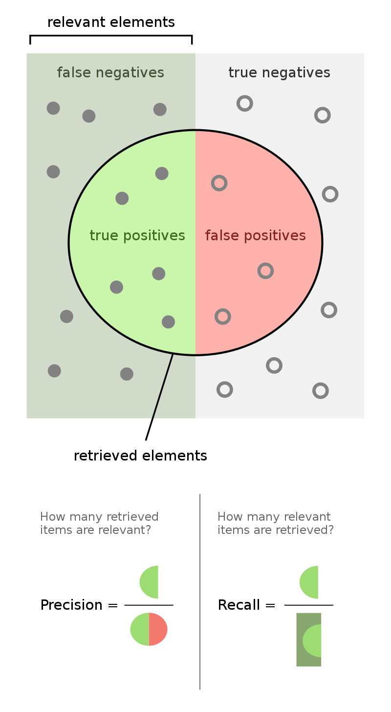
Precision and recall

$$\text{precision} = \frac{TP}{TP + FP} \: \: \: \: \: \: \: \: \text{recall} = \frac{TP}{TP + FN}$$

Question 🤔 (Answer at dsc80.com/q)

Code: pvsr

🤔 When might high precision be more important than high recall?

🤔 When might high recall be more important than high precision?

Question 🤔 (Answer at dsc80.com/q)

Code: billy22

Taken from the Spring 2022 Final Exam.

After fitting a BillyClassifier, we use it to make predictions on an unseen test set. Our results are summarized in the following confusion matrix.

	Predicted Negative	Predicted Positive
Actually Negative	???	30
Actually Positive	66	105

Part 1: What is the recall of our classifier? Give your answer as a fraction (it does not need to be simplified).

Part 2: The accuracy of our classifier is $\frac{69}{117}$. How many true negatives did our classifier have? Give your answer as an integer.

Part 3: True or False: In order for a binary classifier's precision and recall to be equal, the number of mistakes it makes must be an even number.

Part 4: Suppose we are building a classifier that listens to an audio source (say, from your phone’s microphone) and predicts whether or not it is Soulja Boy’s 2008 classic “Kiss Me thru the Phone." Our classifier is pretty good at detecting when the input stream is ”Kiss Me thru the Phone", but it often incorrectly predicts that similar sounding songs are also “Kiss Me thru the Phone."

Complete the sentence: Our classifier has...

• low precision and low recall.
• low precision and high recall.
• high precision and low recall.
• high precision and high recall.

Logistic regression

Wisconsin breast cancer dataset

The Wisconsin breast cancer dataset (WBCD) is a commonly-used dataset for demonstrating binary classification. It is built into sklearn.datasets.

from sklearn.datasets import load_breast_cancer
loaded = load_breast_cancer() # explore the value of `loaded`!
data = loaded['data']
labels = 1 - loaded['target']
cols = loaded['feature_names']
bc = pd.DataFrame(data, columns=cols)

bc.head()

	mean radius	mean texture	mean perimeter	mean area	...	worst concavity	worst concave points	worst symmetry	worst fractal dimension
0	17.990	10.380	122.800	1001.000	...	0.712	0.265	0.460	0.119
1	20.570	17.770	132.900	1326.000	...	0.242	0.186	0.275	0.089
2	19.690	21.250	130.000	1203.000	...	0.450	0.243	0.361	0.088
3	11.420	20.380	77.580	386.100	...	0.687	0.258	0.664	0.173
4	20.290	14.340	135.100	1297.000	...	0.400	0.163	0.236	0.077

5 rows × 30 columns

1 stands for "malignant", i.e. cancerous, and 0 stands for "benign", i.e. safe.

labels

array([1, 1, 1, ..., 1, 1, 0])

pd.Series(labels).value_counts(normalize=True)

0   0.627
1   0.373
Name: proportion, dtype: float64

Our goal is to use the features in bc to predict labels.

Logistic regression

Logistic regression is a linear classification technique that builds upon linear regression. It models the probability of belonging to class 1, given a feature vector:

$$P(y = 1 | \vec{x}) = \sigma (\underbrace{w_0 + w_1 x^{(1)} + w_2 x^{(2)} + ... + w_d x^{(d)}}_{\text{linear regression model}})$$

Here, $\sigma(t) = \frac{1}{1 + e^{-t}}$ is the sigmoid function; its outputs are between 0 and 1 (which means they can be interpreted as probabilities).

🤔 Question: Suppose our logistic regression model predicts the probability that a tumor is malignant is 0.75. What class do we predict – malignant or benign? What if the predicted probability is 0.3?

🙋 Answer: We have to pick a threshold (e.g. 0.5)!

• If the predicted probability is above the threshold, we predict malignant (1).
• Otherwise, we predict benign (0).
• In practice, we use cross validation to decide this threshold.

Fitting a logistic regression model

from sklearn.model_selection import train_test_split
from sklearn.linear_model import LogisticRegression

X_train, X_test, y_train, y_test = train_test_split(bc, labels)

clf = LogisticRegression(max_iter=10000)
clf.fit(X_train, y_train)

LogisticRegression(max_iter=10000)

In a Jupyter environment, please rerun this cell to show the HTML representation or trust the notebook.
On GitHub, the HTML representation is unable to render, please try loading this page with nbviewer.org.

How did clf come up with 1s and 0s?

clf.predict(X_test)

array([1, 0, 0, ..., 0, 1, 0])

It turns out that the predicted labels come from applying a threshold of 0.5 to the predicted probabilities. We can access the predicted probabilities using the predict_proba method:

# [:, 1] refers to the predicted probabilities for class 1.
clf.predict_proba(X_test)

array([[0.  , 1.  ],
       [1.  , 0.  ],
       [0.98, 0.02],
       ...,
       [1.  , 0.  ],
       [0.  , 1.  ],
       [1.  , 0.  ]])

Note that our model still has $w^*$s:

clf.intercept_

array([-30.45])

clf.coef_

array([[-0.97, -0.09,  0.28, ...,  0.48,  0.64,  0.07]])

Evaluating our model

Let's see how well our model does on the test set.

from sklearn import metrics

y_pred = clf.predict(X_test)

Which metric is more important for this task – precision or recall?

metrics.confusion_matrix(y_test, y_pred)

array([[91,  1],
       [ 6, 45]])

from sklearn.metrics import ConfusionMatrixDisplay
ConfusionMatrixDisplay.from_estimator(clf, X_test, y_test);
plt.grid(False)

metrics.accuracy_score(y_test, y_pred)

0.951048951048951

metrics.precision_score(y_test, y_pred)

np.float64(0.9782608695652174)

metrics.recall_score(y_test, y_pred)

np.float64(0.8823529411764706)

What if we choose a different threshold?

🤔 Question: Suppose we choose a threshold higher than 0.5. What will happen to our model's precision and recall?

🙋 Answer: Precision will increase, while recall will decrease*.

• If the "bar" is higher to predict 1, then we will have fewer positives in general, and thus fewer false positives.

• The denominator in $\text{precision} = \frac{TP}{TP + FP}$ will get smaller, and so precision will increase.

• However, the number of false negatives will increase, as we are being more "strict" about what we classify as positive, and so $\text{recall} = \frac{TP}{TP + FN}$ will decrease.

• *It is possible for either or both to stay the same, if changing the threshold slightly (e.g. from 0.5 to 0.500001) doesn't change any predictions.

Similarly, if we decrease our threshold, our model's precision will decrease, while its recall will increase.

Trying several thresholds

The classification threshold is not actually a hyperparameter of LogisticRegression, because the threshold doesn't change the coefficients ($w^*$s) of the logistic regression model itself (see this article for more details).

• Still, the threshold affects our decision rule, so we can tune it using cross-validation (which is not what we're doing below).
• It's also useful to plot how our metrics change as we change the threshold.

thresholds = np.arange(0.01, 1.01, 0.01)
precisions = np.array([])
recalls = np.array([])

for t in thresholds:
    y_pred = clf.predict_proba(X_test)[:, 1] >= t
    precisions = np.append(precisions, metrics.precision_score(y_test, y_pred, zero_division=1))
    recalls = np.append(recalls, metrics.recall_score(y_test, y_pred))

Let's visualize the results.

px.line(x=thresholds, y=precisions,
        labels={'x': 'Threshold', 'y': 'Precision'}, title='Precision vs. Threshold', width=1000, height=600)

px.line(x=thresholds, y=recalls, 
        labels={'x': 'Threshold', 'y': 'Recall'}, title='Recall vs. Threshold', width=1000, height=600)

px.line(x=recalls, y=precisions, hover_name=thresholds, 
        labels={'x': 'Recall', 'y': 'Precision'}, title='Precision vs. Recall')

The above curve is called a precision-recall (or PR) curve.

🤔 Question: Based on the PR curve above, what threshold would you choose?

Combining precision and recall

If we care equally about a model's precision $PR$ and recall $RE$, we can combine the two using a single metric called the F1-score:

$$\text{F1-score} = \text{harmonic mean}(PR, RE) = 2\frac{PR \cdot RE}{PR + RE}$$

pr = metrics.precision_score(y_test, clf.predict(X_test))
re = metrics.recall_score(y_test, clf.predict(X_test))

2 * pr * re / (pr + re)

np.float64(0.9278350515463919)

metrics.f1_score(y_test, clf.predict(X_test))

np.float64(0.9278350515463918)

Both F1-score and accuracy are overall measures of a binary classifier's performance. But remember, accuracy is misleading in the presence of class imbalance, and doesn't take into account the kinds of errors the classifier makes.

metrics.accuracy_score(y_test, clf.predict(X_test))

0.951048951048951

Other evaluation metrics for binary classifiers

We just scratched the surface! This excellent table from Wikipedia summarizes the many other metrics that exist.

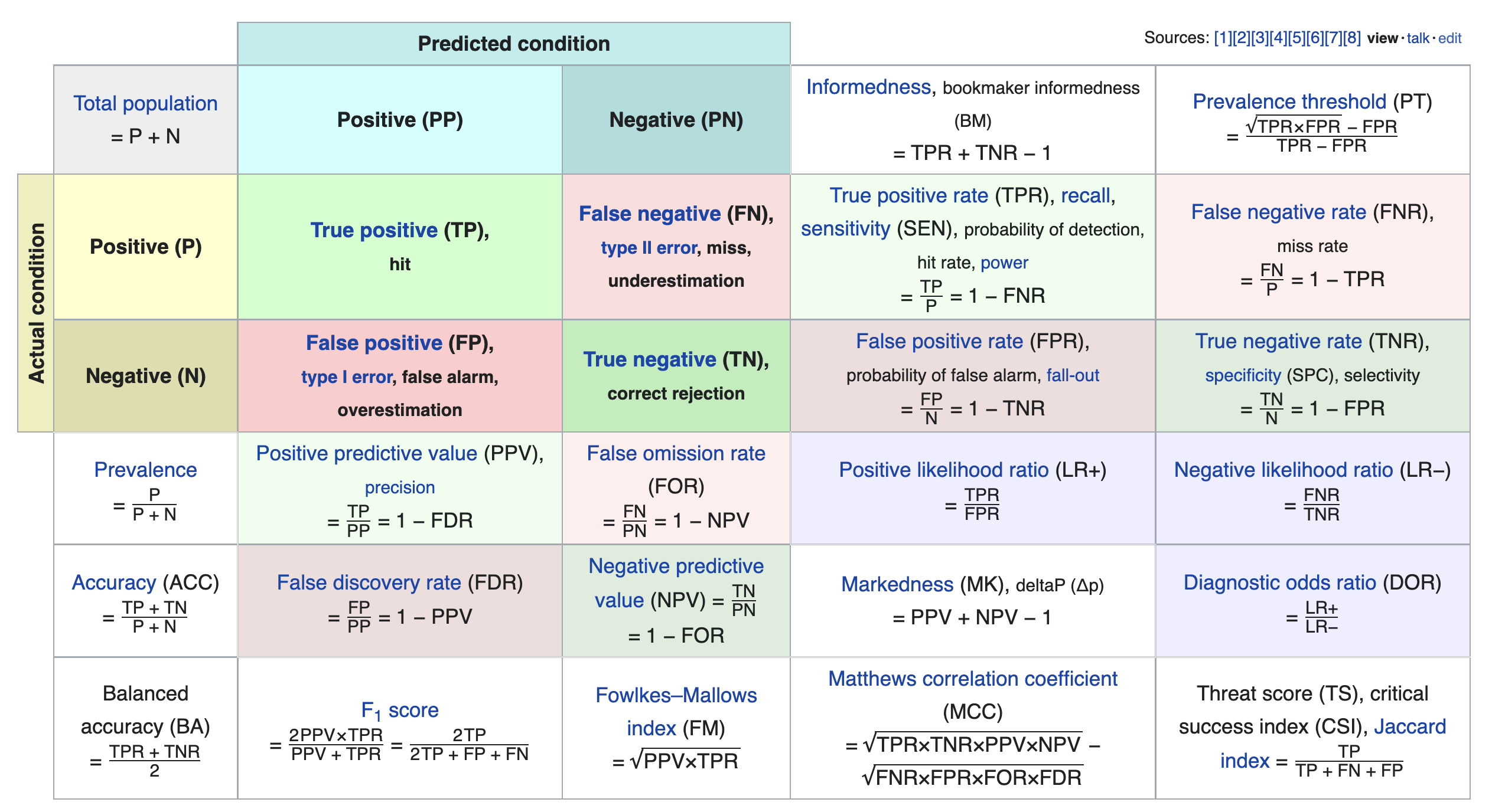
If you're interested in exploring further, a good next metric to look at is true negative rate (i.e. specificity), which is the analogue of recall for true negatives.

Model fairness

Fairness: why do we care?

• Sometimes, a model performs better for certain groups than others; in such cases we say the model is unfair.

• Since ML models are now used in processes that significantly affect human lives, it is important that they are fair!
  • Job applications and college admissions.
  • Criminal sentencing and parole grants.
  • Predictive policing.
  • Credit and loans.

Model fairness

• We'd like to build a model that is fair, meaning that it performs the same for individuals within a group and individuals outside of the group.

• What do we mean by "perform"? What do we mean by "the same"?

Parity measures for classifiers

Suppose $C$ is a classifier we've already trained, and $A$ is some binary attribute that denotes whether an individual is a member of a sensitive group – that is, a group we want to avoid discrimination for (e.g. $A = \text{age is less than 25}$).

• $C$ achieves accuracy parity if $C$ has the same accuracy for individuals in $A$ and individuals not in $A$.
  • Example: $C$ is a binary classifier that determines whether someone receives a loan.
    • If the classifier predicts correctly, then either $C$ approves the loan and it is paid off, or $C$ denies the loan and it would have defaulted.
    • If $C$ achieves accuracy parity, then the proportion of correctly classified loans should be the same for those under 25 and those over 25.

• $C$ achieves precision (or recall) parity if $C$ has the same precision (or recall) for individuals in $A$ and individuals not in $A$.
  • Recall parity is often called "true positive rate parity."

• $C$ achieves demographic parity if the proportion of predictions that are positive is equal for individuals in $A$ and individuals not in $A$.

• With the exception of demographic parity, the parity measures above all involve checking whether some evaluation metric from Lecture 17 is equal across two groups.

More on parity measures

• Which parity metric should you care about? It depends on your specific dataset and what types of errors are important!

• Many of these parity measures are impossible to satisfy simultaneously!

• The classifier parity metrics mentioned on the previous slide are only a few of the many possible parity metrics. See these DSC 167 notes for more details, including more formal explanations.

• These don't apply for regression models; for those, we may care about RMSE parity or $R^2$ parity. There is also a notion of demographic parity for regression models, but it is outside of the scope of DSC 80.

Example: Loan approval

As you know from Project 2, LendingClub was a "peer-to-peer lending company"; they used to publish a dataset describing the loans that they approved.

• 'tag': whether loan was repaid in full (1.0) or defaulted (0.0).
• 'loan_amnt': amount of the loan in dollars.
• 'emp_length': number of years employed.
• 'home_ownership': whether borrower owns (1.0) or rents (0.0).
• 'inq_last_6mths': number of credit inquiries in last six months.
• 'revol_bal': revolving balance on borrows accounts.
• 'age': age in years of the borrower (protected attribute).

loans = pd.read_csv(Path('data') / 'loan_vars1.csv', index_col=0)
loans.head()

	loan_amnt	emp_length	home_ownership	inq_last_6mths	revol_bal	age	tag
268309	6400.000	0.000	1.000	1.000	899.000	22.000	0.000
301093	10700.000	10.000	1.000	0.000	29411.000	19.000	0.000
1379211	15000.000	10.000	1.000	2.000	9911.000	48.000	0.000
486795	15000.000	10.000	1.000	2.000	15883.000	35.000	0.000
1481134	22775.000	3.000	1.000	0.000	17008.000	39.000	0.000

The total amount of money loaned was over 5 billion dollars!

loans['loan_amnt'].sum()

np.float64(5706507225.0)

loans.shape[0]

386772

Predicting 'tag'

Let's build a classifier that predicts whether or not a loan was paid in full. If we were a bank, we could use our trained classifier to determine whether to approve someone for a loan!

from sklearn.model_selection import train_test_split
from sklearn.ensemble import RandomForestClassifier

X = loans.drop('tag', axis=1)
y = loans.tag
X_train, X_test, y_train, y_test = train_test_split(X, y)

clf = RandomForestClassifier(n_estimators=50)
clf.fit(X_train, y_train)

RandomForestClassifier(n_estimators=50)

In a Jupyter environment, please rerun this cell to show the HTML representation or trust the notebook.
On GitHub, the HTML representation is unable to render, please try loading this page with nbviewer.org.

Recall, a prediction of 1 means that we predict that the loan will be paid in full.

y_pred = clf.predict(X_test)
y_pred

array([0., 1., 0., ..., 1., 1., 0.])

clf.score(X_test, y_test)

0.7142088879236346

ConfusionMatrixDisplay.from_estimator(clf, X_test, y_test);
plt.grid(False)

Precision

$$\text{precision} = \frac{TP}{TP+FP}$$

Precision describes the proportion of loans that were approved that would have been paid back.

metrics.precision_score(y_test, y_pred)

np.float64(0.7727873911605864)

If we subtract the precision from 1, we get the proportion of loans that were approved that would not have been paid back. This is known as the false discovery rate.

$$\frac{FP}{TP + FP} = 1 - \text{precision}$$

1 - metrics.precision_score(y_test, y_pred)

np.float64(0.22721260883941363)

Recall

$$\text{recall} = \frac{TP}{TP + FN}$$

Recall describes the proportion of loans that would have been paid back that were actually approved.

metrics.recall_score(y_test, y_pred)

np.float64(0.7337530958942338)

If we subtract the recall from 1, we get the proportion of loans that would have been paid back that were denied. This is known as the false negative rate.

$$\frac{FN}{TP + FN} = 1 - \text{recall}$$

1 - metrics.recall_score(y_test, y_pred)

np.float64(0.26624690410576624)

From both the perspective of the bank and the lendee, a high false negative rate is bad!

• The bank left money on the table – the lendee would have paid back the loan, but they weren't approved for a loan.
• The lendee deserved the loan, but weren't given one.

False negative rate by age

results = X_test
results['age_bracket'] = results['age'].apply(lambda x: 5 * (x // 5 + 1))
results['prediction'] = y_pred
results['tag'] = y_test

(
    results
    .groupby('age_bracket')
    [['tag', 'prediction']]
    .apply(lambda x: 1 - metrics.recall_score(x['tag'], x['prediction']))
    .plot(kind='bar', title='False Negative Rate by Age Group')
)

Computing parity measures

• $C$: Our random forest classifier (1 if we approved the loan, 0 if we denied it).
• $A$: Whether or not they were under 25 (1 if under, 0 if above).

results['is_young'] = (results['age'] < 25).replace({True: 'young', False: 'old'})

First, let's compute the proportion of loans that were approved in each group. If these two numbers are the same, $C$ achieves demographic parity.

results.groupby('is_young')['prediction'].mean()

is_young
old     0.686
young   0.295
Name: prediction, dtype: float64

$C$ evidently does not achieve demographic parity – older people are approved for loans far more often! Note that this doesn't factor in whether they were correctly approved or incorrectly approved.

Now, let's compute the accuracy of $C$ in each group. If these two numbers are the same, $C$ achieves accuracy parity.

compute_accuracy = lambda x: metrics.accuracy_score(x['tag'], x['prediction'])

(
    results
    .groupby('is_young')
    [['tag', 'prediction']]
    .apply(compute_accuracy)
    .rename('accuracy')
)

is_young
old     0.730
young   0.679
Name: accuracy, dtype: float64

Hmm... These numbers look much more similar than before!

Is this difference in accuracy significant?

Let's run a permutation test to see if the difference in accuracy is significant.

• Null Hypothesis: The classifier's accuracy is the same for both young people and old people, and any differences are due to chance.
• Alternative Hypothesis: The classifier's accuracy is higher for old people.
• Test statistic: Difference in accuracy (young minus old).
• Significance level: 0.01.

obs = (results
       .groupby('is_young')
       [['tag', 'prediction']]
       .apply(compute_accuracy)
       .diff()
       .iloc[-1])
obs

np.float64(-0.05127926116930481)

diff_in_acc = []
for _ in range(500):
    s = (
        results[['is_young', 'prediction', 'tag']]
        .assign(is_young=np.random.permutation(results['is_young']))
        .groupby('is_young')
        [['tag', 'prediction']]
        .apply(compute_accuracy)
        .diff()
        .iloc[-1]
    )
    
    diff_in_acc.append(s)

fig = pd.Series(diff_in_acc).plot(kind='hist', histnorm='probability', nbins=20,
                            title='Difference in Accuracy (Young - Old)')
fig.add_vline(x=obs, line_color='red')
fig.update_layout(xaxis_range=[-0.1, 0.05])

It seems like the difference in accuracy across the two groups is significant, despite being only ~5%. Thus, $C$ likely does not achieve accuracy parity.

Ethical questions of fairness

Question 🤔 (Answer at dsc80.com/q)

Code: fair

• Question: Is it "fair" to deny loans to younger people at a higher rate?
• Make an argument for "yes", then make an argument for "no".

• Federal law prevents age from being used as a determining factor in denying a loan.

Not only should we use 'age' to determine whether or not to approve a loan, but we also shouldn't use other features that are strongly correlated with 'age', like 'emp_length'.

loans

	loan_amnt	emp_length	home_ownership	inq_last_6mths	revol_bal	age	tag
268309	6400.000	0.000	1.000	1.000	899.000	22.000	0.000
301093	10700.000	10.000	1.000	0.000	29411.000	19.000	0.000
1379211	15000.000	10.000	1.000	2.000	9911.000	48.000	0.000
...	...	...	...	...	...	...	...
1150493	5000.000	1.000	1.000	0.000	3842.000	52.000	1.000
686485	6000.000	10.000	0.000	0.000	6529.000	36.000	1.000
342901	15000.000	8.000	1.000	1.000	16060.000	39.000	1.000

386772 rows × 7 columns

Summary, next time

Summary

• A logistic regression model makes classifications by first predicting a probability and then thresholding that probability.
  • The default threshold is 0.5; by moving the threshold, we change the balance between precision and recall.
• To assess the parity of your model:
  • Choose an evaluation metric, e.g. precision, recall, or accuracy for classifiers, or RMSE or $R^2$ for regressors.
  • Choose a sensitive binary attribute, e.g. "age < 25" or "is data science major", that divides your data into two groups.
  • Conduct a permutation test to verify whether your model's evaluation criteria is similar for individuals in both groups.

Next time

Career advice and exam review!