from dsc80_utils import *

# Pandas Tutor setup
%reload_ext pandas_tutor
%set_pandas_tutor_options {"maxDisplayCols": 8, "nohover": True, "projectorMode": True}

Lecture 3 – Aggregating

DSC 80, Spring 2024

Announcements 📣

• Lab 1 is due tomorrow at 11:59pm.
  • The Welcome Survey is part of your Lab 1; we won't count your Lab 1 as submitted unless your Welcome Survey is also submitted.
• Project 1 is released.
  • The checkpoint (Questions 1-7) is due on Friday, April 12th.
  • The full project is due on Friday, April 19th.
• Lab 2 will be released by tomorrow.

Agenda

• Adding and modifying columns
• Data granularity and the groupby method.
• DataFrameGroupBy objects and aggregation.
• Other DataFrameGroupBy methods.
• Pivot tables using the pivot_table method.

You will need to code a lot today – make sure to pull the course repository

I will code a lot too, and will post my filled-in slides after class.

Question 🤔 (Answer at q.dsc80.com)

Remember, you can always ask questions at q.dsc80.com!

A question for you now: Have you set up your development environment? Have you started on Lab 1?

• A. Yes, I have set up my development environment. I've started Lab 1.
• B. Yes, I have set up my development environment. I haven't started Lab 1.
• C. No, I have not set up my development environment.

Adding and modifying columns

Adding and modifying columns, using a copy

• To add a new column to a DataFrame, use the assign method.
  • To change the values in a column, add a new column with the same name as the existing column.
• Like most pandas methods, assign returns a new DataFrame.
  • Pro ✅: This doesn't inadvertently change any existing variables.
  • Con ❌: It is not very space efficient, as it creates a new copy each time it is called.

dogs = pd.read_csv(Path('data') / 'dogs43.csv', index_col='breed')

dogs.assign(cost_per_year=dogs['lifetime_cost'] / dogs['longevity'])

dogs

💡 Pro-Tip: Method chaining

Chain methods together instead of writing long, hard-to-read lines.

# Finds the rows corresponding to the five cheapest to own breeds on a per-year basis.
dogs.assign(cost_per_year=dogs['lifetime_cost'] / dogs['longevity']).sort_values('cost_per_year').iloc[:5]

💡 Pro-Tip: assign for column names with special characters

You can also use assign when the desired column name has spaces (and other special characters) by unpacking a dictionary:

dogs.assign(**{'cost per year 💵': dogs['lifetime_cost'] / dogs['longevity']})

Adding and modifying columns, in-place

• You can assign a new column to a DataFrame in-place using [].
  • This works like dictionary assignment.
  • This modifies the underlying DataFrame, unlike assign, which returns a new DataFrame.
• This is the more "common" way of adding/modifying columns.
  • ⚠️ Warning: Exercise caution when using this approach, since this approach changes the values of existing variables.

# By default, .copy() returns a deep copy of the object it is called on,
# meaning that if you change the copy the original remains unmodified.
dogs_copy = dogs.copy()
dogs_copy.head(2)

dogs_copy['cost_per_year'] = dogs_copy['lifetime_cost'] / dogs_copy['longevity']
dogs_copy

Note that we never reassigned dogs_copy in the cell above – that is, we never wrote dogs_copy = ... – though it was still modified.

Mutability

DataFrames, like lists, arrays, and dictionaries, are mutable. As you learned in DSC 20, this means that they can be modified after being created. (For instance, the list .append method mutates in-place.)

Not only does this explain the behavior on the previous slide, but it also explains the following:

dogs_copy

def cost_in_thousands():
    dogs_copy['lifetime_cost'] = dogs_copy['lifetime_cost'] / 1000

# What happens when we run this twice?
cost_in_thousands()

dogs_copy

⚠️ Avoid mutation when possible

Note that dogs_copy was modified, even though we didn't reassign it! These unintended consequences can influence the behavior of test cases on labs and projects, among other things!

To avoid this, it's a good idea to avoid mutation when possible. If you must use mutation, include df = df.copy() as the first line in functions that take DataFrames as input.

Also, some methods let you use the inplace=True argument to mutate the original. Don't use this argument, since future pandas releases plan to remove it.

pandas and numpy

pandas is built upon numpy!

• A Series in pandas is a numpy array with an index.
• A DataFrame is like a dictionary of columns, each of which is a numpy array.
• Many operations in pandas are fast because they use numpy's implementations, which are written in fast languages like C.
• If you need access the array underlying a DataFrame or Series, use the to_numpy method.

dogs['lifetime_cost']

dogs['lifetime_cost'].to_numpy()

Axes

• The rows and columns of a DataFrame are both stored as Series.
• The axis specifies the direction of a slice of a DataFrame.

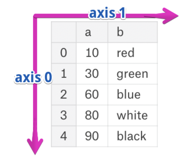
• Axis 0 refers to the index (rows).
• Axis 1 refers to the columns.
• These are the same axes definitions that 2D numpy arrays have!

DataFrame methods with axis

• Many Series methods work on DataFrames.
• In such cases, the DataFrame method usually applies the Series method to every row or column.
• Many of these methods accept an axis argument; the default is usually axis=0.

dogs

# Max element in each column.
dogs.max()

# Max element in each row – a little nonsensical, since there are different types in each row.
dogs.max(axis=1)

# The number of unique values in each column.
dogs.nunique()

# describe doesn't accept an axis argument; it works on every numeric column in the DataFrame it is called on.
dogs.describe()

Data granularity and the groupby method

Example: Palmer Penguins

Artwork by @allison_horst

The dataset we'll work with for the rest of the lecture involves various measurements taken of three species of penguins in Antarctica.

IFrame('https://www.youtube-nocookie.com/embed/CCrNAHXUstU?si=-DntSyUNp5Kwitjm&start=11',
       width=560, height=315)

import seaborn as sns
penguins = sns.load_dataset('penguins').dropna()
penguins

Here, each row corresponds to a single penguin, and each column corresponds to a different attribute (or feature) we have for each penguin. Data formatted in this way is called tidy data.

Granularity

• Granularity refers to what each observation in a dataset represents.
  • Fine: small details.
  • Coarse: bigger picture.

• If you can control how your dataset is created, you should opt for finer granularity, i.e. for more detail.
  • You can always remove details, but it's difficult to add detail that isn't already there.
  • But obtaining fine-grained data can take more time/money.

• Today, we'll focus on how to remove details from fine-grained data, in order to help us understand bigger-picture trends in our data.

Aggregating

Aggregating is the act of combining many values into a single value.

• What is the mean 'body_mass_g' for all penguins?

penguins['body_mass_g'].mean()

• What is the mean 'body_mass_g' for each species?

# ???

Naive approach: looping through unique values

species_map = pd.Series([], dtype=float)

for species in penguins['species'].unique():
    species_only = penguins.loc[penguins['species'] == species]
    species_map.loc[species] = species_only['body_mass_g'].mean()
    
species_map

• For each unique 'species', we make a pass through the entire dataset.
  • The asymptotic runtime of this procedure is $\Theta(ns)$, where $n$ is the number of rows and $s$ is the number of unique species.

• While there are other loop-based solutions that only involve a single pass over the DataFrame, we'd like to avoid Python loops entirely, as they're slow.

Grouping

A better solution, as we know from DSC 10, is to use the groupby method.

# Before:
penguins['body_mass_g'].mean()

# After:
penguins.groupby('species')['body_mass_g'].mean()

Somehow, the groupby method computes what we're looking for in just one line. How?

%%pt

penguins.groupby('species')['body_mass_g'].mean()

"Split-apply-combine" paradigm

The groupby method involves three steps: split, apply, and combine. This is the same terminology that the pandas documentation uses.

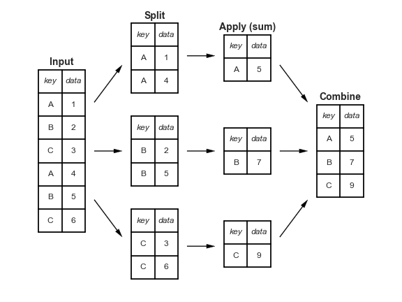
• Split breaks up and "groups" the rows of a DataFrame according to the specified key. There is one "group" for every unique value of the key.

• Apply uses a function (e.g. aggregation, transformation, filtration) within the individual groups.

• Combine stitches the results of these operations into an output DataFrame.

• The split-apply-combine pattern can be parallelized to work on multiple computers or threads, by sending computations for each group to different processors.

More examples

Before we dive into the internals, let's look at a few more examples.

Question 🤔 (Answer at q.dsc80.com)

What proportion of penguins of each 'species' live on 'Dream' island?

Your output should look like:

species
Adelie       0.38
Chinstrap    1.00
Gentoo       0.00

# Fill this in, then respond on q.dsc80.com

DataFrameGroupBy objects and aggregation

DataFrameGroupBy objects

We've just evaluated a few expressions of the following form.

penguins.groupby('species').mean()

There are two method calls in the expression above: .groupby('species') and .mean(). What happens if we remove the latter?

penguins.groupby('species')

Peeking under the hood

If df is a DataFrame, then df.groupby(key) returns a DataFrameGroupBy object.

This object represents the "split" in "split-apply-combine".

# Simplified DataFrame for demonstration:
penguins_small = penguins.iloc[[0, 150, 300, 1, 251, 151, 301], [0, 5, 6]]
penguins_small

# Creates one group for each unique value in the species column.
penguin_groups = penguins_small.groupby('species')
penguin_groups

%%pt
penguin_groups

DataFrameGroupBy objects have a groups attribute, which is a dictionary in which the keys are group names and the values are lists of row labels.

penguin_groups.groups

DataFrameGroupBy objects also have a get_group(key) method, which returns a DataFrame with only the values for the given key.

penguin_groups.get_group('Chinstrap')

# Same as the above!
penguins_small.query('species == "Chinstrap"')

We usually don't use these attributes and methods, but they're useful in understanding how groupby works under the hood.

Aggregation

• Once we create a DataFrameGroupBy object, we need to apply some function to each group, and combine the results.

• The most common operation we apply to each group is an aggregation.

  • Remember, aggregation is the act of combining many values into a single value.

• To perform an aggregation, use an aggregation method on the DataFrameGroupBy object, e.g. .mean(), .max(), or .median().

Let's look at some examples.

penguins_small

penguins_small.groupby('species').mean()

penguins_small.groupby('species').sum()

penguins_small.groupby('species').last()

penguins_small.groupby('species').max()

Column independence

Within each group, the aggregation method is applied to each column independently.

penguins_small.groupby('species').max()

It is not telling us that there is a 'Male' 'Adelie' penguin with a 'body_mass_g' of 3800.0!

# This penguin is Female!
penguins_small.loc[(penguins['species'] == 'Adelie') & (penguins['body_mass_g'] == 3800.0)]

Question 🤔 (Answer at q.dsc80.com)

Find the 'species' and 'body_mass_g' of the heaviest 'Male' and 'Female' penguins in penguins (not penguins_small).

# Your code goes here.

Column selection and performance implications

• By default, the aggregator will be applied to all columns that it can be applied to.
  • max and min are defined on strings, while median and mean are not.

• If we only care about one column, we can select that column before aggregating to save time.
  • DataFrameGroupBy objects support [] notation, just like DataFrames.

# Back to the big penguins dataset!
penguins.groupby('species').mean()

# Works, but involves wasted effort since the other columns had to be aggregated for no reason.
penguins.groupby('species').mean()['bill_length_mm']

# This is a SeriesGroupBy object!
penguins.groupby('species')['bill_length_mm']

# Saves time!
penguins.groupby('species')['bill_length_mm'].mean()

To demonstrate that the former is slower than the latter, we can use %%timeit. For reference, we'll also include our earlier for-loop-based solution.

%%timeit
penguins.groupby('species').mean()['bill_length_mm']

%%timeit
penguins.groupby('species')['bill_length_mm'].mean()

%%timeit
species_map = pd.Series([], dtype=float)

for species in penguins['species'].unique():
    species_only = penguins.loc[penguins['species'] == species]
    species_map.loc[species] = species_only['body_mass_g'].mean()
    
species_map

Takeaways

• It's important to understand what each piece of your code evaluates to – in the first two timed examples, the code is almost identical, but the performance is quite different.

  # Slower
  penguins.groupby('species').mean()['bill_length_mm']
  
  # Faster
  penguins.groupby('species')['bill_length_mm'].mean()
  

• The groupby method is much quicker than for-looping over the DataFrame in Python. It can often produce results using just a single, fast pass over the data, updating the sum, mean, count, min, or other aggregate for each group along the way.

Beyond default aggregation methods

• There are many built-in aggregation methods.
• What if you want to apply different aggregation methods to different columns?
• What if the aggregation method you want to use doesn't already exist in pandas?

The aggregate method

• The DataFrameGroupBy object has a general aggregate method, which aggregates using one or more operations.
  • Remember, aggregation is the act of combining many values into a single value.
• There are many ways of using aggregate; refer to the documentation for a comprehensive list.
• Example arguments:
  • A single function.
  • A list of functions.
  • A dictionary mapping column names to functions.
• Per the documentation, agg is an alias for aggregate.

Example

How many penguins are there of each 'species', and what is the mean 'body_mass_g' of each 'species'?

(penguins
 .groupby('species')
 ['body_mass_g']
 .aggregate(['count', 'mean'])
)

Note what happens when we don't select a column before aggregating.

(penguins
 .groupby('species')
 .aggregate(['count', 'mean'])
)

Example

What is the maximum 'bill_length_mm' of each 'species', and which 'island's is each 'species' found on?

(penguins
 .groupby('species')
 .aggregate({'bill_length_mm': 'max', 'island': 'unique'})
)

Example

What is the interquartile range of the 'body_mass_g' of each 'species'?

# Here, the argument to agg is a function,
# which takes in a pd.Series and returns a scalar.

def iqr(s):
    return np.percentile(s, 75) - np.percentile(s, 25)

(penguins
 .groupby('species')
 ['body_mass_g']
 .agg(iqr)
)

Question 🤔 (Answer at q.dsc80.com)

What questions do you have?

Other DataFrameGroupBy methods

Split-apply-combine, revisited

When we introduced the split-apply-combine pattern, the "apply" step involved aggregation – our final DataFrame had one row for each group.

Instead of aggregating during the apply step, we could instead perform a:

• Transformation, in which we perform operations to every value within each group.

• Filtration, in which we keep only the groups that satisfy some condition.

Transformations

Suppose we want to convert the 'body_mass_g' column to to z-scores (i.e. standard units):

$$z(x_i) = \frac{x_i - \text{mean of } x}{\text{SD of } x}$$

def z_score(x):
    return (x - x.mean()) / x.std(ddof=0)

z_score(penguins['body_mass_g'])

Transformations within groups

• Now, what if we wanted the z-score within each group?

• To do so, we can use the transform method on a DataFrameGroupBy object. The transform method takes in a function, which itself takes in a Series and returns a new Series.

• A transformation produces a DataFrame or Series of the same size – it is not an aggregation!

z_mass = (penguins
          .groupby('species')
          ['body_mass_g']
          .transform(z_score))
z_mass

penguins.assign(z_mass=z_mass)

display_df(penguins.assign(z_mass=z_mass), rows=8)

Note that above, penguin 340 has a larger 'body_mass_g' than penguin 0, but a lower 'z_mass'.

• Penguin 0 has an above average 'body_mass_g' among 'Adelie' penguins.
• Penguin 340 has a below average 'body_mass_g' among 'Gentoo' penguins. Remember from earlier that the average 'body_mass_g' of 'Gentoo' penguins is much higher than for other species.

penguins.groupby('species')['body_mass_g'].mean()

Filtering groups

• To keep only the groups that satisfy a particular condition, use the filter method on a DataFrameGroupBy object.

• The filter method takes in a function, which itself takes in a DataFrame/Series and return a single Boolean. The result is a new DataFrame/Series with only the groups for which the filter function returned True.

For example, suppose we want only the 'species' whose average 'bill_length_mm' is above 39.

(penguins
 .groupby('species')
 .filter(lambda df: df['bill_length_mm'].mean() > 39)
)

No more 'Adelie's!

Or, as another example, suppose we only want 'species' with at least 100 penguins:

(penguins
 .groupby('species')
 .filter(lambda df: df.shape[0] > 100)
)

No more 'Chinstrap's!

Question 🤔 (Answer at q.dsc80.com)

Answer the following questions about grouping:

• In .agg(fn), what is the input to fn? What is the output of fn?
• In .transform(fn), what is the input to fn? What is the output of fn?
• In .filter(fn), what is the input to fn? What is the output of fn?

Grouping with multiple columns

When we group with multiple columns, one group is created for every unique combination of elements in the specified columns.

species_and_island = penguins.groupby(['species', 'island']).mean()
species_and_island

Grouping and indexes

• The groupby method creates an index based on the specified columns.
• When grouping by multiple columns, the resulting DataFrame has a MultiIndex.
• Advice: When working with a MultiIndex, use reset_index or set as_index=False in groupby.

species_and_island

species_and_island['body_mass_g']

species_and_island.loc['Adelie']

species_and_island.loc[('Adelie', 'Torgersen')]

species_and_island.reset_index()

penguins.groupby(['species', 'island'], as_index=False).mean()

Question 🤔 (Answer at q.dsc80.com)

Find the most popular 'Male' and 'Female' baby 'Name' for each 'Year' in baby. Exclude 'Year's where there were fewer than 1 million births recorded.

baby_path = Path('data') / 'baby.csv'
baby = pd.read_csv(baby_path)
baby

# Your code goes here.

Pivot tables using the pivot_table method

Pivot tables: an extension of grouping

Pivot tables are a compact way to display tables for humans to read:

Sex	F	M
Year
2018	1698373	1813377
2019	1675139	1790682
2020	1612393	1721588
2021	1635800	1743913
2022	1628730	1733166

• Notice that each value in the table is a sum over the counts, split by year and sex.
• You can think of pivot tables as grouping using two columns, then "pivoting" one of the group labels into columns.

pivot_table

The pivot_table DataFrame method aggregates a DataFrame using two columns. To use it:

df.pivot_table(index=index_col,
               columns=columns_col,
               values=values_col,
               aggfunc=func)

The resulting DataFrame will have:

• One row for every unique value in index_col.
• One column for every unique value in columns_col.
• Values determined by applying func on values in values_col.

last_5_years = baby.query('Year >= 2018')
last_5_years

last_5_years.pivot_table(
    index='Year',
    columns='Sex',
    values='Count',
    aggfunc='sum',
)

# Look at the similarity to the snippet above!
(last_5_years
 .groupby(['Year', 'Sex'])
 [['Count']]
 .sum()
)

Example

Find the number of penguins per 'island' and 'species'.

penguins

penguins.pivot_table(
    index='species', 
    columns='island', 
    values='bill_length_mm', # Choice of column here doesn't actually matter!
    aggfunc='count',
)

Note that there is a NaN at the intersection of 'Biscoe' and 'Chinstrap', because there were no Chinstrap penguins on Biscoe Island.

We can either use the fillna method afterwards or the fill_value argument to fill in NaNs.

penguins.pivot_table(
    index='species', 
    columns='island', 
    values='bill_length_mm', 
    aggfunc='count',
    fill_value=0,
)

Granularity, revisited

Take another look at the pivot table from the previous slide. Each row of the original penguins DataFrame represented a single penguin, and each column represented features of the penguins.

What is the granularity of the DataFrame below?

penguins.pivot_table(
    index='species', 
    columns='island', 
    values='bill_length_mm', 
    aggfunc='count',
    fill_value=0,
)

Reshaping

• pivot_table reshapes DataFrames from "long" to "wide".
• Other DataFrame reshaping methods:
  • melt: Un-pivots a DataFrame. Very useful in data cleaning.
  • pivot: Like pivot_table, but doesn't do aggregation.
  • stack: Pivots multi-level columns to multi-indices.
  • unstack: Pivots multi-indices to columns.
  • Google and the documentation are your friends!

Question 🤔 (Answer at q.dsc80.com)

What questions do you have?

Distributions

Joint distribution

When using aggfunc='count', a pivot table describes the joint distribution of two categorical variables. This is also called a contingency table.

counts = penguins.pivot_table(
    index='species', 
    columns='sex', 
    values='body_mass_g', 
    aggfunc='count', 
    fill_value=0
)
counts

We can normalize the DataFrame by dividing by the total number of penguins. The resulting numbers can be interpreted as probabilities that a randomly selected penguin from the dataset belongs to a given combination of species and sex.

joint = counts / counts.sum().sum()
joint

Marginal probabilities

If we sum over one of the axes, we can compute marginal probabilities, i.e. unconditional probabilities.

joint

# Recall, joint.sum(axis=0) sums across the rows, 
# which computes the sum of the **columns**.
joint.sum(axis=0)

joint.sum(axis=1)

For instance, the second Series tells us that a randomly selected penguin has a 0.36 chance of being of species 'Gentoo'.

Conditional probabilities

Using counts, how might we compute conditional probabilities like $$P(\text{species } = \text{"Adelie"} \mid \text{sex } = \text{"Female"})?$$

counts

$$\begin{align*} P(\text{species} = c \mid \text{sex} = x) &= \frac{\# \: (\text{species} = c \text{ and } \text{sex} = x)}{\# \: (\text{sex} = x)} \end{align*}$$

➡️ Click here to see more of a derivation.

$$\begin{align*} P(\text{species} = c \mid \text{sex} = x) &= \frac{P(\text{species} = c \text{ and } \text{sex} = x)}{P(\text{sex = }x)} \\ &= \frac{\frac{\# \: (\text{species } = \: c \text{ and } \text{sex } = \: x)}{N}}{\frac{\# \: (\text{sex } = \: x)}{N}} \\ &= \frac{\# \: (\text{species} = c \text{ and } \text{sex} = x)}{\# \: (\text{sex} = x)} \end{align*}$$

Answer: To find conditional probabilities of 'species' given 'sex', divide by column sums. To find conditional probabilities of 'sex' given 'species', divide by row sums.

Conditional probabilities

To find conditional probabilities of 'species' given 'sex', divide by column sums. To find conditional probabilities of 'sex' given 'species', divide by row sums.

counts

counts.sum(axis=0)

The conditional distribution of 'species' given 'sex' is below. Note that in this new DataFrame, the 'Female' and 'Male' columns each sum to 1.

counts / counts.sum(axis=0)

For instance, the above DataFrame tells us that the probability that a randomly selected penguin is of 'species' 'Adelie' given that they are of 'sex' 'Female' is 0.442424.

Question 🤔 (Answer at q.dsc80.com)

Find the conditional distribution of 'sex' given 'species'.

Hint: Use .T.

# Your code goes here.

Summary, next time

Summary

• Grouping allows us to change the level of granularity in a DataFrame.
• Grouping involves three steps – split, apply, and combine.
  • Usually, what is applied is an aggregation, but it could be a transformation or filtration.
• pivot_table aggregates data based on two categorical columns, and reshapes the result to be "wide" instead of "long".

Next time

• Simpson's paradox.
• Merging.
  • Review this diagram from DSC 10!
• The pitfalls of the apply method.