# You'll start seeing this cell in most lectures.
# It exists to hide all of the import statements and other setup
# code we need in lecture notebooks.
from dsc80_utils import *

Pre-Lecture Reading for Lecture 2 – DataFrame Fundamentals

DSC 80, Winter 2024

Make sure to read this before attending lecture (which, remember, is on Zoom today.)

You can also access this notebook by pulling the course GitHub repository and opening lectures/lec02/pre-lec02.ipynb.

In this reading, we'll review some of the basics of numpy and babypandas that you're familiar with from DSC 10. In lecture, we'll build off of this foundation.

numpy arrays

numpy overview

• numpy stands for "numerical Python". It is a commonly-used Python module that enables fast computation involving arrays and matrices.
• numpy's main object is the array. In numpy, arrays are:
  • Homogenous – all values are of the same type.
  • (Potentially) multi-dimensional.
• Computation in numpy is fast because:
  • Much of it is implemented in C.
  • numpy arrays are stored more efficiently in memory than, say, Python lists.
• This site provides a good overview of numpy arrays.

We used numpy in DSC 10 to work with sequences of data:

arr = np.arange(10)
arr

array([0, 1, 2, 3, 4, 5, 6, 7, 8, 9])

# The shape (10,) means that the array only has a single dimension,
# of size 10.
arr.shape

(10,)

2 ** arr

array([  1,   2,   4,   8,  16,  32,  64, 128, 256, 512])

Arrays come equipped with several handy methods; some examples are below, but you can read about them all here.

(2 ** arr).sum()

1023

(2 ** arr).mean()

102.3

(2 ** arr).max()

512

(2 ** arr).argmax()

9

⚠️ The dangers of for-loops

• for-loops are slow when processing large datasets. You will rarely write for-loops in DSC 80 (except for Lab 1 and Project 1), and may be penalized on assignments for using them when unnecessary!
• One of the biggest benefits of numpy is that it supports vectorized operations.
  • If a and b are two arrays of the same length, then a + b is a new array of the same length containing the element-wise sum of a and b.
• To illustrate how much faster numpy arithmetic is than using a for-loop, let's compute the squares of the numbers between 0 and 1,000,000:
  • Using a for-loop.
  • Using vectorized arithmetic, through numpy.

%%timeit
squares = []
for i in range(1_000_000):
    squares.append(i * i)

47.6 ms ± 526 µs per loop (mean ± std. dev. of 7 runs, 10 loops each)

In vanilla Python, this takes about 0.04 seconds per loop.

%%timeit
squares = np.arange(1_000_000) ** 2

1.46 ms ± 77.1 µs per loop (mean ± std. dev. of 7 runs, 1,000 loops each)

In numpy, this only takes about 0.001 seconds per loop, more than 40x faster! Note that under the hood, numpy is also using a for-loop, but it's a for-loop implemented in C, which is much faster than Python.

Multi-dimensional arrays

While we didn't see these very often in DSC 10, multi-dimensional lists/arrays may have since come up in DSC 20, 30, or 40A (especially in the context of linear algebra).

We'll spend a bit of time talking about 2D (and 3D) arrays here, since in some ways, they behave similarly to DataFrames.

Below, we create a 2D array from scratch.

nums = np.array([
    [5, 1, 9, 7],
    [9, 8, 2, 3],
    [2, 5, 0, 4]
])

nums

array([[5, 1, 9, 7],
       [9, 8, 2, 3],
       [2, 5, 0, 4]])

# nums has 3 rows and 4 columns.
nums.shape

(3, 4)

We can also create 2D arrays by reshaping other arrays.

# Here, we're asking to reshape np.arange(1, 7)
# so that it has 2 rows and 3 columns.
a = np.arange(1, 7).reshape((2, 3))
a

array([[1, 2, 3],
       [4, 5, 6]])

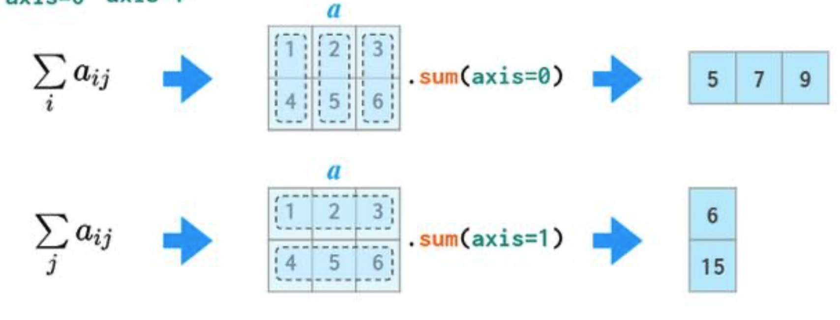
Operations along axes

In 2D arrays (and DataFrames), axis 0 refers to the rows (up and down) and axis 1 refers to the columns (left and right).

a

array([[1, 2, 3],
       [4, 5, 6]])

If we specify axis=0, a.sum will "compress" along axis 0.

a.sum(axis=0)

array([5, 7, 9])

If we specify axis=1, a.sum will "compress" along axis 1.

a.sum(axis=1)

array([ 6, 15])

Selecting rows and columns from 2D arrays

You can use [square brackets] to slice rows and columns out of an array, using the same slicing conventions you saw in DSC 20.

a

array([[1, 2, 3],
       [4, 5, 6]])

# Accesses row 0 and all columns.
a[0, :]

array([1, 2, 3])

# Same as the above.
a[0]

array([1, 2, 3])

# Accesses all rows and column 1.
a[:, 1]

array([2, 5])

# Accesses row 0 and columns 1 and onwards.
a[0, 1:]

array([2, 3])

Exercise

Try and predict the value of grid[-1, 1:].sum() without running the code below.

s = (5, 3)
grid = np.ones(s) * 2 * np.arange(1, 16).reshape(s)
# grid[-1, 1:].sum()

From babypandas to pandas 🐼

babypandas

In DSC 10, you used babypandas, which was a subset of pandas designed to be friendly for beginners.

pandas

You're not a beginner anymore – you've taken DSC 20, 30, and 40A. You're ready for the real deal.

Fortunately, everything you learned in babypandas will carry over!

pandas

• pandas is the Python library for tabular data manipulation.
• Before pandas was developed, the standard data science workflow involved using multiple languages (Python, R, Java) in a single project.
• Wes McKinney, the original developer of pandas, wanted a library which would allow everything to be done in Python.
  • Python is faster to develop in than Java, and is more general-purpose than R.

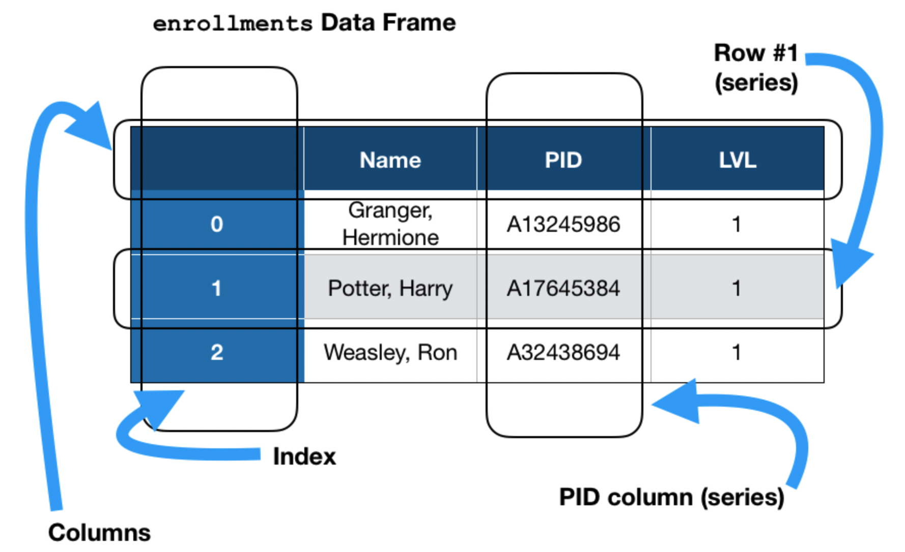
pandas data structures

There are three key data structures at the core of pandas:

• DataFrame: 2 dimensional tables.
• Series: 1 dimensional array-like object, typically representing a column or row.
• Index: sequence of column or row labels.

Importing pandas and related libraries

pandas is almost always imported in conjunction with numpy.

import pandas as pd
import numpy as np

Example: Dog Breeds (woof!) 🐶

We'll provide more context for the dataset we're working with in lecture. For now, all you need to know is that each row corresponds to a different dog breed.

# You'll see the Path(...) / syntax a lot.
# It creates the correct path to your file, 
# whether you're using Windows, macOS, or Linux.
# (Note that macOS and Linux use / to denote separate folders in paths,
# while Windows uses \.)
dog_path = Path('data') / 'dogs43.csv'
dogs = pd.read_csv(dog_path)
dogs

	breed	kind	lifetime_cost	longevity	size	weight	height
0	Brittany	sporting	22589.0	12.92	medium	35.0	19.0
1	Cairn Terrier	terrier	21992.0	13.84	small	14.0	10.0
2	English Cocker Spaniel	sporting	18993.0	11.66	medium	30.0	16.0
...	...	...	...	...	...	...	...
40	Bullmastiff	working	13936.0	7.57	large	115.0	25.5
41	Mastiff	working	13581.0	6.50	large	175.0	30.0
42	Saint Bernard	working	20022.0	7.78	large	155.0	26.5

43 rows × 7 columns

Review: head, tail, shape, index, get, and sort_values

To extract the first or last few rows of a DataFrame, use the head or tail methods.

dogs.head(3)

	breed	kind	lifetime_cost	longevity	size	weight	height
0	Brittany	sporting	22589.0	12.92	medium	35.0	19.0
1	Cairn Terrier	terrier	21992.0	13.84	small	14.0	10.0
2	English Cocker Spaniel	sporting	18993.0	11.66	medium	30.0	16.0

dogs.tail(2)

	breed	kind	lifetime_cost	longevity	size	weight	height
41	Mastiff	working	13581.0	6.50	large	175.0	30.0
42	Saint Bernard	working	20022.0	7.78	large	155.0	26.5

The shape attribute returns the DataFrame's number of rows and columns.

dogs.shape

(43, 7)

# The default index of a DataFrame is 0, 1, 2, 3, ...
dogs.index

RangeIndex(start=0, stop=43, step=1)

We know that we can use .get() to select out a column or multiple columns...

dogs.get('breed')

0                   Brittany
1              Cairn Terrier
2     English Cocker Spaniel
               ...          
40               Bullmastiff
41                   Mastiff
42             Saint Bernard
Name: breed, Length: 43, dtype: object

dogs.get(['breed', 'kind', 'longevity'])

	breed	kind	longevity
0	Brittany	sporting	12.92
1	Cairn Terrier	terrier	13.84
2	English Cocker Spaniel	sporting	11.66
...	...	...	...
40	Bullmastiff	working	7.57
41	Mastiff	working	6.50
42	Saint Bernard	working	7.78

43 rows × 3 columns

Most people don't use .get in practice; we'll see the more common technique in lecture.

And lastly, remember that to sort by a column, use the sort_values method. Like most DataFrame and Series methods, sort_values returns a new DataFrame, and doesn't modify the original.

# Note that the index is no longer 0, 1, 2, ...!
dogs.sort_values('height', ascending=False)

	breed	kind	lifetime_cost	longevity	size	weight	height
41	Mastiff	working	13581.0	6.50	large	175.0	30.0
36	Borzoi	hound	16176.0	9.08	large	82.5	28.0
34	Newfoundland	working	19351.0	9.32	large	125.0	27.0
...	...	...	...	...	...	...	...
29	Dandie Dinmont Terrier	terrier	21633.0	12.17	small	21.0	9.0
14	Maltese	toy	19084.0	12.25	small	5.0	9.0
8	Chihuahua	toy	26250.0	16.50	small	5.5	5.0

43 rows × 7 columns

# This sorts by 'height', 
# then breaks ties by 'longevity'.
# Note the difference in the last three rows between
# this DataFrame and the one above.
dogs.sort_values(['height', 'longevity'],
                 ascending=False)

	breed	kind	lifetime_cost	longevity	size	weight	height
41	Mastiff	working	13581.0	6.50	large	175.0	30.0
36	Borzoi	hound	16176.0	9.08	large	82.5	28.0
34	Newfoundland	working	19351.0	9.32	large	125.0	27.0
...	...	...	...	...	...	...	...
14	Maltese	toy	19084.0	12.25	small	5.0	9.0
29	Dandie Dinmont Terrier	terrier	21633.0	12.17	small	21.0	9.0
8	Chihuahua	toy	26250.0	16.50	small	5.5	5.0

43 rows × 7 columns

Note that dogs is not the DataFrame above. To save our changes, we'd need to say something like dogs = dogs.sort_values....

dogs

	breed	kind	lifetime_cost	longevity	size	weight	height
0	Brittany	sporting	22589.0	12.92	medium	35.0	19.0
1	Cairn Terrier	terrier	21992.0	13.84	small	14.0	10.0
2	English Cocker Spaniel	sporting	18993.0	11.66	medium	30.0	16.0
...	...	...	...	...	...	...	...
40	Bullmastiff	working	13936.0	7.57	large	115.0	25.5
41	Mastiff	working	13581.0	6.50	large	175.0	30.0
42	Saint Bernard	working	20022.0	7.78	large	155.0	26.5

43 rows × 7 columns

That's all we need to review... we'll pick back up in lecture!