from dsc80_utils import *
# Pandas Tutor setup
%reload_ext pandas_tutor
%set_pandas_tutor_options {"maxDisplayCols": 8, "nohover": True, "projectorMode": True}
Lecture 3 – Grouping and Pivoting
DSC 80, Winter 2024
There was a (very short) Pre-Lecture Reading for this lecture – we'll assume you've done it.
Announcements 📣
- Lab 1 is due tomorrow at 5PM. You cannot use slip days on it!
- Please fill out the Welcome Survey if you haven't already!
- Project 1 is released.
- The checkpoint (Questions 1-7) is due on Saturday, January 20th.
- The full project is due on Saturday, January 27th.
- Lab 2 will be released by tomorrow.
Agenda
- Data granularity and the
groupbymethod. DataFrameGroupByobjects and aggregation.- Other
DataFrameGroupBymethods. - Pivot tables using the
pivot_tablemethod.
You will need to code a lot today – make sure to pull the course repository
I will code a lot too, and will post my filled-in slides after class.
Question 🤔 (Answer at q.dsc80.com)
Remember, you can always ask questions at q.dsc80.com!
A question for you now: did you look at the pre-lecture reading diagram? Have you set up your development environment?
- A. Yes, I looked at the pre-lecture reading. Yes, I have set up my development environment.
- B. Yes, I looked at the pre-lecture reading. No, I have not set up my development environment.
- C. No, I did not look at the pre-lecture reading. Yes, I have set up my development environment.
- D. No, I did not look at the pre-lecture reading. No, I have not set up my development environment.
Data granularity and the groupby method
Example: Palmer Penguins
 Artwork by @allison_horst
The dataset we'll work with for the rest of the lecture involves various measurements taken of three species of penguins in Antarctica.
IFrame('https://www.youtube-nocookie.com/embed/CCrNAHXUstU?si=-DntSyUNp5Kwitjm&start=11',
       width=560, height=315)
import seaborn as sns
penguins = sns.load_dataset('penguins').dropna()
penguins
| species | island | bill_length_mm | bill_depth_mm | flipper_length_mm | body_mass_g | sex | |
|---|---|---|---|---|---|---|---|
| 0 | Adelie | Torgersen | 39.1 | 18.7 | 181.0 | 3750.0 | Male |
| 1 | Adelie | Torgersen | 39.5 | 17.4 | 186.0 | 3800.0 | Female |
| 2 | Adelie | Torgersen | 40.3 | 18.0 | 195.0 | 3250.0 | Female |
| ... | ... | ... | ... | ... | ... | ... | ... |
| 341 | Gentoo | Biscoe | 50.4 | 15.7 | 222.0 | 5750.0 | Male |
| 342 | Gentoo | Biscoe | 45.2 | 14.8 | 212.0 | 5200.0 | Female |
| 343 | Gentoo | Biscoe | 49.9 | 16.1 | 213.0 | 5400.0 | Male |
333 rows × 7 columns
Here, each row corresponds to a single penguin, and each column corresponds to a different attribute (or feature) we have for each penguin. Data formatted in this way is called tidy data.
Granularity
- Granularity refers to what each observation in a dataset represents.
- Fine: small details.
- Coarse: bigger picture.
- If you can control how your dataset is created, you should opt for finer granularity, i.e. for more detail.
- You can always remove details, but it's difficult to add detail that isn't already there.
- But obtaining fine-grained data can take more time/money.
- Today, we'll focus on how to remove details from fine-grained data, in order to help us understand bigger-picture trends in our data.
Initial exploration
Given our penguins dataset, we may wonder:
- What is the distribution of
'species'in this dataset?
penguins['species'].value_counts()
Adelie       146
Gentoo       119
Chinstrap     68
Name: species, dtype: int64
penguins['species'].value_counts(normalize=True)
Adelie       0.44
Gentoo       0.36
Chinstrap    0.20
Name: species, dtype: float64
- What is the distribution of
'islands'?
penguins['island'].value_counts()
Biscoe       163
Dream        123
Torgersen     47
Name: island, dtype: int64
Aggregating
Aggregating is the act of combining many values into a single value.
- What is the mean
'body_mass_g'for all penguins?
penguins['body_mass_g'].mean()
4207.057057057057
- What is the mean
'body_mass_g'for each species?
# ???
Naive approach: looping through unique values
species_map = pd.Series([], dtype=float)

for species in penguins['species'].unique():
    species_only = penguins.loc[penguins['species'] == species]
    species_map.loc[species] = species_only['body_mass_g'].mean()

species_map
Adelie       3706.16
Chinstrap    3733.09
Gentoo       5092.44
dtype: float64
- For each unique
'species', we make a pass through the entire dataset.- The asymptotic runtime of this procedure is $\Theta(ns)$, where $n$ is the number of rows and $s$ is the number of unique species.
- While there are other loop-based solutions that only involve a single pass over the DataFrame, we'd like to avoid Python loops entirely, as they're slow.
Grouping
A better solution, as we know from DSC 10, is to use the groupby method.
# Before:
penguins['body_mass_g'].mean()
4207.057057057057
# After:
penguins.groupby('species').mean()['body_mass_g']
species
Adelie       3706.16
Chinstrap    3733.09
Gentoo       5092.44
Name: body_mass_g, dtype: float64
Somehow, the groupby method computes what we're looking for in just one line. How?
%%pt

penguins.groupby('species').mean()['body_mass_g']
"Split-apply-combine" paradigm
The groupby method involves three steps: split, apply, and combine. This is the same terminology that the pandas documentation uses.
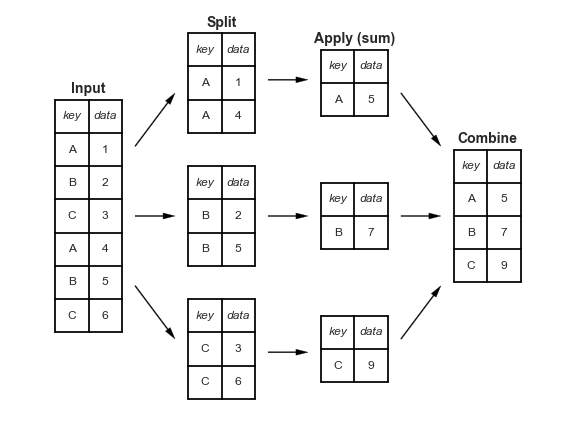
Split breaks up and "groups" the rows of a DataFrame according to the specified key. There is one "group" for every unique value of the key.
Apply uses a function (e.g. aggregation, transformation, filtration) within the individual groups.
Combine stitches the results of these operations into an output DataFrame.
The split-apply-combine pattern can be parallelized to work on multiple computers or threads, by sending computations for each group to different processors.
More examples
Before we dive into the internals, let's look at a few more examples.
penguins
| species | island | bill_length_mm | bill_depth_mm | flipper_length_mm | body_mass_g | sex | |
|---|---|---|---|---|---|---|---|
| 0 | Adelie | Torgersen | 39.1 | 18.7 | 181.0 | 3750.0 | Male |
| 1 | Adelie | Torgersen | 39.5 | 17.4 | 186.0 | 3800.0 | Female |
| 2 | Adelie | Torgersen | 40.3 | 18.0 | 195.0 | 3250.0 | Female |
| ... | ... | ... | ... | ... | ... | ... | ... |
| 341 | Gentoo | Biscoe | 50.4 | 15.7 | 222.0 | 5750.0 | Male |
| 342 | Gentoo | Biscoe | 45.2 | 14.8 | 212.0 | 5200.0 | Female |
| 343 | Gentoo | Biscoe | 49.9 | 16.1 | 213.0 | 5400.0 | Male |
333 rows × 7 columns
Exercise
Which'species' has the highest median 'bill_length_mm'?
penguins
| species | island | bill_length_mm | bill_depth_mm | flipper_length_mm | body_mass_g | sex | |
|---|---|---|---|---|---|---|---|
| 0 | Adelie | Torgersen | 39.1 | 18.7 | 181.0 | 3750.0 | Male |
| 1 | Adelie | Torgersen | 39.5 | 17.4 | 186.0 | 3800.0 | Female |
| 2 | Adelie | Torgersen | 40.3 | 18.0 | 195.0 | 3250.0 | Female |
| ... | ... | ... | ... | ... | ... | ... | ... |
| 341 | Gentoo | Biscoe | 50.4 | 15.7 | 222.0 | 5750.0 | Male |
| 342 | Gentoo | Biscoe | 45.2 | 14.8 | 212.0 | 5200.0 | Female |
| 343 | Gentoo | Biscoe | 49.9 | 16.1 | 213.0 | 5400.0 | Male |
333 rows × 7 columns
# Your code goes here.
penguins.groupby('species').median()['bill_length_mm'].idxmax()
'Chinstrap'
What proportion of penguins of each 'species' live on 'Dream' island?
(
    penguins
    .assign(is_dream=penguins['island'] == 'Dream')
    .groupby('species')
    .mean()
    ['is_dream']
)
species
Adelie       0.38
Chinstrap    1.00
Gentoo       0.00
Name: is_dream, dtype: float64
DataFrameGroupBy objects and aggregation
DataFrameGroupBy objects
We've just evaluated a few expressions of the following form.
penguins.groupby('species').mean()
| bill_length_mm | bill_depth_mm | flipper_length_mm | body_mass_g | |
|---|---|---|---|---|
| species | ||||
| Adelie | 38.82 | 18.35 | 190.10 | 3706.16 |
| Chinstrap | 48.83 | 18.42 | 195.82 | 3733.09 |
| Gentoo | 47.57 | 15.00 | 217.24 | 5092.44 |
There are two method calls in the expression above: .groupby('species') and .mean(). What happens if we remove the latter?
penguins.groupby('species')
<pandas.core.groupby.generic.DataFrameGroupBy object at 0x15ceb5ac0>
Peeking under the hood
If df is a DataFrame, then df.groupby(key) returns a DataFrameGroupBy object.
This object represents the "split" in "split-apply-combine".
# Simplified DataFrame for demonstration:
penguins_small = penguins.iloc[[0, 150, 300, 1, 251, 151, 301], [0, 5, 6]]
penguins_small
| species | body_mass_g | sex | |
|---|---|---|---|
| 0 | Adelie | 3750.0 | Male |
| 156 | Chinstrap | 3725.0 | Male |
| 308 | Gentoo | 4875.0 | Female |
| 1 | Adelie | 3800.0 | Female |
| 258 | Gentoo | 4350.0 | Female |
| 157 | Chinstrap | 3950.0 | Female |
| 309 | Gentoo | 5550.0 | Male |
# Creates one group for each unique value in the species column.
penguin_groups = penguins_small.groupby('species')
penguin_groups
<pandas.core.groupby.generic.DataFrameGroupBy object at 0x15ceb58b0>
%%pt
penguin_groups
DataFrameGroupBy objects have a groups attribute, which is a dictionary in which the keys are group names and the values are lists of row labels.
penguin_groups.groups
{'Adelie': [0, 1], 'Chinstrap': [156, 157], 'Gentoo': [308, 258, 309]}
DataFrameGroupBy objects also have a get_group(key) method, which returns a DataFrame with only the values for the given key.
penguin_groups.get_group('Chinstrap')
| species | body_mass_g | sex | |
|---|---|---|---|
| 156 | Chinstrap | 3725.0 | Male |
| 157 | Chinstrap | 3950.0 | Female |
# Same as the above!
penguins_small.query('species == "Chinstrap"')
| species | body_mass_g | sex | |
|---|---|---|---|
| 156 | Chinstrap | 3725.0 | Male |
| 157 | Chinstrap | 3950.0 | Female |
We usually don't use these attributes and methods, but they're useful in understanding how groupby works under the hood.
Aggregation
Once we create a
DataFrameGroupByobject, we need to apply some function to each group, and combine the results.The most common operation we apply to each group is an aggregation.
- Remember, aggregation is the act of combining many values into a single value.
To perform an aggregation, use an aggregation method on the
DataFrameGroupByobject, e.g..mean(),.max(), or.median().
Let's look at some examples.
penguins_small
| species | body_mass_g | sex | |
|---|---|---|---|
| 0 | Adelie | 3750.0 | Male |
| 156 | Chinstrap | 3725.0 | Male |
| 308 | Gentoo | 4875.0 | Female |
| 1 | Adelie | 3800.0 | Female |
| 258 | Gentoo | 4350.0 | Female |
| 157 | Chinstrap | 3950.0 | Female |
| 309 | Gentoo | 5550.0 | Male |
penguins_small.groupby('species').mean()
| body_mass_g | |
|---|---|
| species | |
| Adelie | 3775.0 |
| Chinstrap | 3837.5 |
| Gentoo | 4925.0 |
penguins_small.groupby('species').sum()
| body_mass_g | |
|---|---|
| species | |
| Adelie | 7550.0 |
| Chinstrap | 7675.0 |
| Gentoo | 14775.0 |
penguins_small
| species | body_mass_g | sex | |
|---|---|---|---|
| 0 | Adelie | 3750.0 | Male |
| 156 | Chinstrap | 3725.0 | Male |
| 308 | Gentoo | 4875.0 | Female |
| 1 | Adelie | 3800.0 | Female |
| 258 | Gentoo | 4350.0 | Female |
| 157 | Chinstrap | 3950.0 | Female |
| 309 | Gentoo | 5550.0 | Male |
penguins_small.groupby('species').last()
| body_mass_g | sex | |
|---|---|---|
| species | ||
| Adelie | 3800.0 | Female |
| Chinstrap | 3950.0 | Female |
| Gentoo | 5550.0 | Male |
penguins_small
| species | body_mass_g | sex | |
|---|---|---|---|
| 0 | Adelie | 3750.0 | Male |
| 156 | Chinstrap | 3725.0 | Male |
| 308 | Gentoo | 4875.0 | Female |
| 1 | Adelie | 3800.0 | Female |
| 258 | Gentoo | 4350.0 | Female |
| 157 | Chinstrap | 3950.0 | Female |
| 309 | Gentoo | 5550.0 | Male |
penguins_small.groupby('species').max()
| body_mass_g | sex | |
|---|---|---|
| species | ||
| Adelie | 3800.0 | Male |
| Chinstrap | 3950.0 | Male |
| Gentoo | 5550.0 | Male |
Column independence
Within each group, the aggregation method is applied to each column independently.
penguins_small.groupby('species').max()
| body_mass_g | sex | |
|---|---|---|
| species | ||
| Adelie | 3800.0 | Male |
| Chinstrap | 3950.0 | Male |
| Gentoo | 5550.0 | Male |
It is not telling us that there is a 'Male' 'Adelie' penguin with a 'body_mass_g' of 3800.0!
# This penguin is Female!
penguins_small.loc[(penguins_small['species'] == 'Adelie') & (penguins_small['body_mass_g'] == 3800.0)]
| species | body_mass_g | sex | |
|---|---|---|---|
| 1 | Adelie | 3800.0 | Female |
Exercise
Find the'species' and 'body_mass_g' of the heaviest 'Male' and 'Female' penguins in penguins (not penguins_small).
# Your code goes here.
(
    penguins
    .sort_values('body_mass_g', ascending=False)
    .groupby('sex')
    .first()
)
| species | island | bill_length_mm | bill_depth_mm | flipper_length_mm | body_mass_g | |
|---|---|---|---|---|---|---|
| sex | ||||||
| Female | Gentoo | Biscoe | 45.2 | 14.8 | 212.0 | 5200.0 |
| Male | Gentoo | Biscoe | 49.2 | 15.2 | 221.0 | 6300.0 |
Column selection and performance implications
- By default, the aggregator will be applied to all columns that it can be applied to.
maxandminare defined on strings, whilemedianandmeanare not.
- If we only care about one column, we can select that column before aggregating to save time.
DataFrameGroupByobjects support[]notation, just likeDataFrames.
# Back to the big penguins dataset!
penguins.groupby('species').mean()
| bill_length_mm | bill_depth_mm | flipper_length_mm | body_mass_g | |
|---|---|---|---|---|
| species | ||||
| Adelie | 38.82 | 18.35 | 190.10 | 3706.16 |
| Chinstrap | 48.83 | 18.42 | 195.82 | 3733.09 |
| Gentoo | 47.57 | 15.00 | 217.24 | 5092.44 |
# Works, but involves wasted effort since the other columns had to be aggregated for no reason.
penguins.groupby('species').mean()['bill_length_mm']
species
Adelie       38.82
Chinstrap    48.83
Gentoo       47.57
Name: bill_length_mm, dtype: float64
# This is a SeriesGroupBy object!
penguins.groupby('species')['bill_length_mm']
<pandas.core.groupby.generic.SeriesGroupBy object at 0x15d8853a0>
# Saves time!
penguins.groupby('species')['bill_length_mm'].mean()
species
Adelie       38.82
Chinstrap    48.83
Gentoo       47.57
Name: bill_length_mm, dtype: float64
To demonstrate that the former is slower than the latter, we can use %%timeit. For reference, we'll also include our earlier for-loop-based solution.
%%timeit
penguins.groupby('species').mean()['bill_length_mm']
302 µs ± 3.96 µs per loop (mean ± std. dev. of 7 runs, 1,000 loops each)
%%timeit
penguins.groupby('species')['bill_length_mm'].mean()
116 µs ± 1.6 µs per loop (mean ± std. dev. of 7 runs, 10,000 loops each)
%%timeit
species_map = pd.Series([], dtype=float)

for species in penguins['species'].unique():
    species_only = penguins.loc[penguins['species'] == species]
    species_map.loc[species] = species_only['body_mass_g'].mean()

species_map
884 µs ± 12.8 µs per loop (mean ± std. dev. of 7 runs, 1,000 loops each)
Takeaways
It's important to understand what each piece of your code evaluates to – in the first two timed examples, the code is almost identical, but the performance is quite different.
# Slower
penguins.groupby('species').mean()['bill_length_mm']

# Faster
penguins.groupby('species')['bill_length_mm'].mean()
The
groupbymethod is much quicker thanfor-looping over the DataFrame in Python. It can often produce results using just a single, fast pass over the data, updating the sum, mean, count, min, or other aggregate for each group along the way.
Beyond default aggregation methods
- There are many built-in aggregation methods.
- What if you want to apply different aggregation methods to different columns?
- What if the aggregation method you want to use doesn't already exist in
pandas?
The aggregate method
- The
DataFrameGroupByobject has a generalaggregatemethod, which aggregates using one or more operations.- Remember, aggregation is the act of combining many values into a single value.
- There are many ways of using
aggregate; refer to the documentation for a comprehensive list. - Example arguments:
- A single function.
- A list of functions.
- A dictionary mapping column names to functions.
- Per the documentation,
aggis an alias foraggregate.
Example
How many penguins are there of each 'species', and what is the mean 'body_mass_g' of each 'species'?
(
    penguins
    .groupby('species')
    ['body_mass_g']
    .aggregate(['count', 'mean'])
)
| count | mean | |
|---|---|---|
| species | ||
| Adelie | 146 | 3706.16 |
| Chinstrap | 68 | 3733.09 |
| Gentoo | 119 | 5092.44 |
Note what happens when we don't select a column before aggregating.
(
    penguins
    .groupby('species')
    .aggregate(['count', 'mean'])
)
| bill_length_mm | bill_depth_mm | flipper_length_mm | body_mass_g | |||||
|---|---|---|---|---|---|---|---|---|
| count | mean | count | mean | count | mean | count | mean | |
| species | ||||||||
| Adelie | 146 | 38.82 | 146 | 18.35 | 146 | 190.10 | 146 | 3706.16 |
| Chinstrap | 68 | 48.83 | 68 | 18.42 | 68 | 195.82 | 68 | 3733.09 |
| Gentoo | 119 | 47.57 | 119 | 15.00 | 119 | 217.24 | 119 | 5092.44 |
Example
What is the maximum 'bill_length_mm' of each 'species', and which 'island's is each 'species' found on?
(
    penguins
    .groupby('species')
    .agg({'bill_length_mm': 'max', 'island': 'unique'})
)
| bill_length_mm | island | |
|---|---|---|
| species | ||
| Adelie | 46.0 | [Torgersen, Biscoe, Dream] |
| Chinstrap | 58.0 | [Dream] |
| Gentoo | 59.6 | [Biscoe] |
Example
What is the interquartile range of the 'body_mass_g' of each 'species'?
# Here, the argument to agg is a function,
# which takes in a pd.Series and returns a scalar.

def iqr(s):
    return np.percentile(s, 75) - np.percentile(s, 25)

(
    penguins
    .groupby('species')
    ['body_mass_g']
    .aggregate(iqr)
)
species
Adelie       637.5
Chinstrap    462.5
Gentoo       800.0
Name: body_mass_g, dtype: float64
Question 🤔 (Answer at q.dsc80.com)
What questions do you have?
Other DataFrameGroupBy methods
Split-apply-combine, revisited
When we introduced the split-apply-combine pattern, the "apply" step involved aggregation – our final DataFrame had one row for each group.
Instead of aggregating during the apply step, we could instead perform a:
Transformation, in which we perform operations to every value within each group.
Filtration, in which we keep only the groups that satisfy some condition.
Transformations
Suppose we want to convert the 'body_mass_g' column to to z-scores (i.e. standard units):
def z_score(x):
    return (x - x.mean()) / x.std(ddof=0) # makes sure that the denominator in standard deviation is n instead of n - 1
z_score(penguins['body_mass_g'])
0     -0.57
1     -0.51
2     -1.19
       ...
341    1.92
342    1.23
343    1.48
Name: body_mass_g, Length: 333, dtype: float64
Transformations within groups
Now, what if we wanted the z-score within each group?
To do so, we can use the
transformmethod on aDataFrameGroupByobject. Thetransformmethod takes in a function, which itself takes in a Series and returns a new Series.A transformation produces a DataFrame or Series of the same size – it is not an aggregation!
z_mass = (
    penguins
    .groupby('species')
    ['body_mass_g']
    .transform(z_score)
)
z_mass
0      0.10
1      0.21
2     -1.00
       ...
341    1.32
342    0.22
343    0.62
Name: body_mass_g, Length: 333, dtype: float64
display_df(penguins.assign(z_mass=z_mass), rows=8)
| species | island | bill_length_mm | bill_depth_mm | flipper_length_mm | body_mass_g | sex | z_mass | |
|---|---|---|---|---|---|---|---|---|
| 0 | Adelie | Torgersen | 39.1 | 18.7 | 181.0 | 3750.0 | Male | 0.10 |
| 1 | Adelie | Torgersen | 39.5 | 17.4 | 186.0 | 3800.0 | Female | 0.21 |
| 2 | Adelie | Torgersen | 40.3 | 18.0 | 195.0 | 3250.0 | Female | -1.00 |
| 4 | Adelie | Torgersen | 36.7 | 19.3 | 193.0 | 3450.0 | Female | -0.56 |
| ... | ... | ... | ... | ... | ... | ... | ... | ... |
| 340 | Gentoo | Biscoe | 46.8 | 14.3 | 215.0 | 4850.0 | Female | -0.49 |
| 341 | Gentoo | Biscoe | 50.4 | 15.7 | 222.0 | 5750.0 | Male | 1.32 |
| 342 | Gentoo | Biscoe | 45.2 | 14.8 | 212.0 | 5200.0 | Female | 0.22 |
| 343 | Gentoo | Biscoe | 49.9 | 16.1 | 213.0 | 5400.0 | Male | 0.62 |
333 rows × 8 columns
penguins.groupby('species')['body_mass_g'].mean()
species
Adelie       3706.16
Chinstrap    3733.09
Gentoo       5092.44
Name: body_mass_g, dtype: float64
Note that above, penguin 340 has a larger 'body_mass_g' than penguin 0, but a lower 'z_mass'.
- Penguin 0 has an above average
'body_mass_g'among'Adelie'penguins. - Penguin 340 has a below average
'body_mass_g'among'Gentoo'penguins. Remember from earlier that the average'body_mass_g'of'Gentoo'penguins is much higher than for other species.
Filtering groups
To keep only the groups that satisfy a particular condition, use the
filtermethod on aDataFrameGroupByobject.The
filtermethod takes in a function, which itself takes in a DataFrame/Series and return a single Boolean. The result is a new DataFrame/Series with only the groups for which the filter function returnedTrue.
For example, suppose we want only the 'species' whose average 'bill_length_mm' is above 39.
(
    penguins
    .groupby('species')
    .filter(lambda df: df['bill_length_mm'].mean() > 39)
)
| species | island | bill_length_mm | bill_depth_mm | flipper_length_mm | body_mass_g | sex | |
|---|---|---|---|---|---|---|---|
| 152 | Chinstrap | Dream | 46.5 | 17.9 | 192.0 | 3500.0 | Female |
| 153 | Chinstrap | Dream | 50.0 | 19.5 | 196.0 | 3900.0 | Male |
| 154 | Chinstrap | Dream | 51.3 | 19.2 | 193.0 | 3650.0 | Male |
| ... | ... | ... | ... | ... | ... | ... | ... |
| 341 | Gentoo | Biscoe | 50.4 | 15.7 | 222.0 | 5750.0 | Male |
| 342 | Gentoo | Biscoe | 45.2 | 14.8 | 212.0 | 5200.0 | Female |
| 343 | Gentoo | Biscoe | 49.9 | 16.1 | 213.0 | 5400.0 | Male |
187 rows × 7 columns
No more 'Adelie's!
Or, as another example, suppose we only want 'species' with at least 100 penguins:
(
    penguins
    .groupby('species')
    .filter(lambda df: df.shape[0] >= 100)
)
| species | island | bill_length_mm | bill_depth_mm | flipper_length_mm | body_mass_g | sex | |
|---|---|---|---|---|---|---|---|
| 0 | Adelie | Torgersen | 39.1 | 18.7 | 181.0 | 3750.0 | Male |
| 1 | Adelie | Torgersen | 39.5 | 17.4 | 186.0 | 3800.0 | Female |
| 2 | Adelie | Torgersen | 40.3 | 18.0 | 195.0 | 3250.0 | Female |
| ... | ... | ... | ... | ... | ... | ... | ... |
| 341 | Gentoo | Biscoe | 50.4 | 15.7 | 222.0 | 5750.0 | Male |
| 342 | Gentoo | Biscoe | 45.2 | 14.8 | 212.0 | 5200.0 | Female |
| 343 | Gentoo | Biscoe | 49.9 | 16.1 | 213.0 | 5400.0 | Male |
265 rows × 7 columns
No more 'Chinstrap's!
Grouping with multiple columns
When we group with multiple columns, one group is created for every unique combination of elements in the specified columns.
species_and_island = penguins.groupby(['species', 'island']).mean()
species_and_island
| bill_length_mm | bill_depth_mm | flipper_length_mm | body_mass_g | ||
|---|---|---|---|---|---|
| species | island | ||||
| Adelie | Biscoe | 38.98 | 18.37 | 188.80 | 3709.66 |
| Dream | 38.52 | 18.24 | 189.93 | 3701.36 | |
| Torgersen | 39.04 | 18.45 | 191.53 | 3708.51 | |
| Chinstrap | Dream | 48.83 | 18.42 | 195.82 | 3733.09 |
| Gentoo | Biscoe | 47.57 | 15.00 | 217.24 | 5092.44 |
Grouping and indexes
- The
groupbymethod creates an index based on the specified columns. - When grouping by multiple columns, the resulting DataFrame has a
MultiIndex. - Advice: When working with a
MultiIndex, usereset_indexor setas_index=Falseingroupby.
species_and_island
| bill_length_mm | bill_depth_mm | flipper_length_mm | body_mass_g | ||
|---|---|---|---|---|---|
| species | island | ||||
| Adelie | Biscoe | 38.98 | 18.37 | 188.80 | 3709.66 |
| Dream | 38.52 | 18.24 | 189.93 | 3701.36 | |
| Torgersen | 39.04 | 18.45 | 191.53 | 3708.51 | |
| Chinstrap | Dream | 48.83 | 18.42 | 195.82 | 3733.09 |
| Gentoo | Biscoe | 47.57 | 15.00 | 217.24 | 5092.44 |
species_and_island['body_mass_g']
species    island
Adelie     Biscoe       3709.66
           Dream        3701.36
           Torgersen    3708.51
Chinstrap  Dream        3733.09
Gentoo     Biscoe       5092.44
Name: body_mass_g, dtype: float64
species_and_island.loc['Adelie']
| bill_length_mm | bill_depth_mm | flipper_length_mm | body_mass_g | |
|---|---|---|---|---|
| island | ||||
| Biscoe | 38.98 | 18.37 | 188.80 | 3709.66 |
| Dream | 38.52 | 18.24 | 189.93 | 3701.36 |
| Torgersen | 39.04 | 18.45 | 191.53 | 3708.51 |
species_and_island.loc[('Adelie', 'Torgersen')]
bill_length_mm         39.04
bill_depth_mm          18.45
flipper_length_mm     191.53
body_mass_g          3708.51
Name: (Adelie, Torgersen), dtype: float64
species_and_island.reset_index()
| species | island | bill_length_mm | bill_depth_mm | flipper_length_mm | body_mass_g | |
|---|---|---|---|---|---|---|
| 0 | Adelie | Biscoe | 38.98 | 18.37 | 188.80 | 3709.66 |
| 1 | Adelie | Dream | 38.52 | 18.24 | 189.93 | 3701.36 |
| 2 | Adelie | Torgersen | 39.04 | 18.45 | 191.53 | 3708.51 |
| 3 | Chinstrap | Dream | 48.83 | 18.42 | 195.82 | 3733.09 |
| 4 | Gentoo | Biscoe | 47.57 | 15.00 | 217.24 | 5092.44 |
penguins.groupby(['species', 'island'], as_index=False).mean()
| species | island | bill_length_mm | bill_depth_mm | flipper_length_mm | body_mass_g | |
|---|---|---|---|---|---|---|
| 0 | Adelie | Biscoe | 38.98 | 18.37 | 188.80 | 3709.66 |
| 1 | Adelie | Dream | 38.52 | 18.24 | 189.93 | 3701.36 |
| 2 | Adelie | Torgersen | 39.04 | 18.45 | 191.53 | 3708.51 |
| 3 | Chinstrap | Dream | 48.83 | 18.42 | 195.82 | 3733.09 |
| 4 | Gentoo | Biscoe | 47.57 | 15.00 | 217.24 | 5092.44 |
Exercise
Find the most popular'Male' and 'Female' baby 'Name' for each 'Year' in baby. Exclude 'Year's where there were fewer than 1 million births recorded.
baby_path = Path('data') / 'baby.csv'
baby = pd.read_csv(baby_path)
baby
| Name | Sex | Count | Year | |
|---|---|---|---|---|
| 0 | Liam | M | 20456 | 2022 |
| 1 | Noah | M | 18621 | 2022 |
| 2 | Olivia | F | 16573 | 2022 |
| ... | ... | ... | ... | ... |
| 2085155 | Wright | M | 5 | 1880 |
| 2085156 | York | M | 5 | 1880 |
| 2085157 | Zachariah | M | 5 | 1880 |
2085158 rows × 4 columns
# Your code goes here.
(
    baby
    .groupby('Year')
    .filter(lambda df: df['Count'].sum() > 1_000_000)
    .sort_values('Count', ascending=False)
    .groupby(['Year', 'Sex'])
    .first()
)
| Name | Count | ||
|---|---|---|---|
| Year | Sex | ||
| 1913 | F | Mary | 36642 |
| M | John | 29329 | |
| 1914 | F | Mary | 45346 |
| ... | ... | ... | ... |
| 2021 | M | Liam | 20365 |
| 2022 | F | Olivia | 16573 |
| M | Liam | 20456 |
220 rows × 2 columns
# Verify your answer!
baby.query('Year == 1913 and Sex == "M"').sort_values('Count')
| Name | Sex | Count | Year | |
|---|---|---|---|---|
| 1980373 | Zenus | M | 5 | 1913 |
| 1980072 | Engelbert | M | 5 | 1913 |
| 1980073 | Ephram | M | 5 | 1913 |
| ... | ... | ... | ... | ... |
| 1973409 | James | M | 20832 | 1913 |
| 1973408 | William | M | 23538 | 1913 |
| 1973407 | John | M | 29329 | 1913 |
3261 rows × 4 columns
Pivot tables using the pivot_table method
Pivot tables: an extension of grouping
Pivot tables are a compact way to display tables for humans to read:
| Sex | F | M |
|---|---|---|
| Year | ||
| 2018 | 1698373 | 1813377 |
| 2019 | 1675139 | 1790682 |
| 2020 | 1612393 | 1721588 |
| 2021 | 1635800 | 1743913 |
| 2022 | 1628730 | 1733166 |
- Notice that each value in the table is a sum over the counts, split by year and sex.
- You can think of pivot tables as grouping using two columns, then "pivoting" one of the group labels into columns.
pivot_table
The pivot_table DataFrame method aggregates a DataFrame using two columns. To use it:
df.pivot_table(index=index_col,
               columns=columns_col,
               values=values_col,
               aggfunc=func)
The resulting DataFrame will have:
- One row for every unique value in
index_col. - One column for every unique value in
columns_col. - Values determined by applying
funcon values invalues_col.
last_5_years = baby.query('Year >= 2018')
last_5_years
| Name | Sex | Count | Year | |
|---|---|---|---|---|
| 0 | Liam | M | 20456 | 2022 |
| 1 | Noah | M | 18621 | 2022 |
| 2 | Olivia | F | 16573 | 2022 |
| ... | ... | ... | ... | ... |
| 159444 | Zyrie | M | 5 | 2018 |
| 159445 | Zyron | M | 5 | 2018 |
| 159446 | Zzyzx | M | 5 | 2018 |
159447 rows × 4 columns
last_5_years.pivot_table(
    index='Year',
    columns='Sex',
    values='Count',
    aggfunc='sum'
)
| Sex | F | M |
|---|---|---|
| Year | ||
| 2018 | 1698373 | 1813377 |
| 2019 | 1675139 | 1790682 |
| 2020 | 1612393 | 1721588 |
| 2021 | 1635800 | 1743913 |
| 2022 | 1628730 | 1733166 |
last_5_years.groupby(['Year', 'Sex'])[['Count']].sum()
| Count | ||
|---|---|---|
| Year | Sex | |
| 2018 | F | 1698373 |
| M | 1813377 | |
| 2019 | F | 1675139 |
| ... | ... | ... |
| 2021 | M | 1743913 |
| 2022 | F | 1628730 |
| M | 1733166 |
10 rows × 1 columns
Example
Find the number of penguins per 'island' and 'species'.
penguins
| species | island | bill_length_mm | bill_depth_mm | flipper_length_mm | body_mass_g | sex | |
|---|---|---|---|---|---|---|---|
| 0 | Adelie | Torgersen | 39.1 | 18.7 | 181.0 | 3750.0 | Male |
| 1 | Adelie | Torgersen | 39.5 | 17.4 | 186.0 | 3800.0 | Female |
| 2 | Adelie | Torgersen | 40.3 | 18.0 | 195.0 | 3250.0 | Female |
| ... | ... | ... | ... | ... | ... | ... | ... |
| 341 | Gentoo | Biscoe | 50.4 | 15.7 | 222.0 | 5750.0 | Male |
| 342 | Gentoo | Biscoe | 45.2 | 14.8 | 212.0 | 5200.0 | Female |
| 343 | Gentoo | Biscoe | 49.9 | 16.1 | 213.0 | 5400.0 | Male |
333 rows × 7 columns
penguins.pivot_table(
    index='species',
    columns='island',
    values='flipper_length_mm',
    aggfunc='count'
)
| island | Biscoe | Dream | Torgersen |
|---|---|---|---|
| species | |||
| Adelie | 44.0 | 55.0 | 47.0 |
| Chinstrap | NaN | 68.0 | NaN |
| Gentoo | 119.0 | NaN | NaN |
Note that there is a NaN at the intersection of 'Biscoe' and 'Chinstrap', because there were no Chinstrap penguins on Biscoe Island.
We can either use the fillna method afterwards or the fill_value argument to fill in NaNs.
penguins.pivot_table(
    index='species',
    columns='island',
    values='flipper_length_mm',
    aggfunc='count',
).fillna(0)
| island | Biscoe | Dream | Torgersen |
|---|---|---|---|
| species | |||
| Adelie | 44.0 | 55.0 | 47.0 |
| Chinstrap | 0.0 | 68.0 | 0.0 |
| Gentoo | 119.0 | 0.0 | 0.0 |
penguins.pivot_table(
    index='species',
    columns='island',
    values='flipper_length_mm',
    aggfunc='count',
    fill_value=0
)
| island | Biscoe | Dream | Torgersen |
|---|---|---|---|
| species | |||
| Adelie | 44 | 55 | 47 |
| Chinstrap | 0 | 68 | 0 |
| Gentoo | 119 | 0 | 0 |
Granularity, revisited
Take another look at the pivot table from the previous slide. Each row of the original penguins DataFrame represented a single penguin, and each column represented features of the penguins.
What is the granularity of the DataFrame below?
penguins.pivot_table(
    index='species',
    columns='island',
    values='flipper_length_mm',
    aggfunc='count',
    fill_value=0
)
| island | Biscoe | Dream | Torgersen |
|---|---|---|---|
| species | |||
| Adelie | 44 | 55 | 47 |
| Chinstrap | 0 | 68 | 0 |
| Gentoo | 119 | 0 | 0 |
Reshaping
pivot_tablereshapes DataFrames from "long" to "wide".- Other DataFrame reshaping methods:
melt: Un-pivots a DataFrame. Very useful in data cleaning.pivot: Likepivot_table, but doesn't do aggregation.stack: Pivots multi-level columns to multi-indices.unstack: Pivots multi-indices to columns.- Google and the documentation are your friends!
Question 🤔 (Answer at q.dsc80.com)
What questions do you have?
Distributions
Joint distribution
When using aggfunc='count', a pivot table describes the joint distribution of two categorical variables. This is also called a contingency table.
counts = penguins.pivot_table(
    index='species',
    columns='sex',
    values='body_mass_g',
    aggfunc='count',
    fill_value=0
)
counts
| sex | Female | Male |
|---|---|---|
| species | ||
| Adelie | 73 | 73 |
| Chinstrap | 34 | 34 |
| Gentoo | 58 | 61 |
We can normalize the DataFrame by dividing by the total number of penguins. The resulting numbers can be interpreted as probabilities that a randomly selected penguin from the dataset belongs to a given combination of species and sex.
joint = counts / counts.sum().sum()
joint
| sex | Female | Male |
|---|---|---|
| species | ||
| Adelie | 0.22 | 0.22 |
| Chinstrap | 0.10 | 0.10 |
| Gentoo | 0.17 | 0.18 |
Marginal probabilities
If we sum over one of the axes, we can compute marginal probabilities, i.e. unconditional probabilities.
joint
| sex | Female | Male |
|---|---|---|
| species | ||
| Adelie | 0.22 | 0.22 |
| Chinstrap | 0.10 | 0.10 |
| Gentoo | 0.17 | 0.18 |
# Recall, joint.sum(axis=0) sums across the rows,
# which computes the sum of the **columns**.
joint.sum(axis=0)
sex
Female    0.5
Male      0.5
dtype: float64
joint.sum(axis=1)
species
Adelie       0.44
Chinstrap    0.20
Gentoo       0.36
dtype: float64
For instance, the second Series tells us that a randomly selected penguin has a 0.36 chance of being of species 'Gentoo'.
Conditional probabilities
Using counts, how might we compute conditional probabilities like $$P(\text{species } = \text{"Adelie"} \mid \text{sex } = \text{"Female"})?$$
counts
| sex | Female | Male |
|---|---|---|
| species | ||
| Adelie | 73 | 73 |
| Chinstrap | 34 | 34 |
| Gentoo | 58 | 61 |
➡️ Click here to see more of a derivation.
$$\begin{align*} P(\text{species} = c \mid \text{sex} = x) &= \frac{P(\text{species} = c \text{ and } \text{sex} = x)}{P(\text{sex = }x)} \\ &= \frac{\frac{\# \: (\text{species } = \: c \text{ and } \text{sex } = \: x)}{N}}{\frac{\# \: (\text{sex } = \: x)}{N}} \\ &= \frac{\# \: (\text{species} = c \text{ and } \text{sex} = x)}{\# \: (\text{sex} = x)} \end{align*}$$Answer: To find conditional probabilities of 'species' given 'sex', divide by column sums. To find conditional probabilities of 'sex' given 'species', divide by row sums.
Conditional probabilities
To find conditional probabilities of 'species' given 'sex', divide by column sums. To find conditional probabilities of 'sex' given 'species', divide by row sums.
counts
| sex | Female | Male |
|---|---|---|
| species | ||
| Adelie | 73 | 73 |
| Chinstrap | 34 | 34 |
| Gentoo | 58 | 61 |
counts.sum(axis=0)
sex
Female    165
Male      168
dtype: int64
The conditional distribution of 'species' given 'sex' is below. Note that in this new DataFrame, the 'Female' and 'Male' columns each sum to 1.
counts / counts.sum(axis=0)
| sex | Female | Male |
|---|---|---|
| species | ||
| Adelie | 0.44 | 0.43 |
| Chinstrap | 0.21 | 0.20 |
| Gentoo | 0.35 | 0.36 |
For instance, the above DataFrame tells us that the probability that a randomly selected penguin is of 'species' 'Adelie' given that they are of 'sex' 'Female' is 0.442424.
Exercise
Find the conditional distribution of'sex' given 'species'.Hint: Use
.T.
# Your code goes here.
Summary, next time
Summary
- Grouping allows us to change the level of granularity in a DataFrame.
- Grouping involves three steps – split, apply, and combine.
- Usually, what is applied is an aggregation, but it could be a transformation or filtration.
pivot_tableaggregates data based on two categorical columns, and reshapes the result to be "wide" instead of "long".
Next time
- Simpson's paradox.
- Merging.
- Review this diagram from DSC 10!
- The pitfalls of the
applymethod.