from dsc80_utils import *
Announcements 📣
- The Project 4 checkpoint is due tonight, and the full project is due on Thursday, March 21st.
- You can use slip days on the checkpoint, but not on the final deadline.
- Lab 9 is due on Monday, March 11th.
- The Final Exam is on Tuesday, March 19th from 3-6PM (room TBD).
- Practice by working through old exams at practice.dsc80.com. Even more exams are there now, including this quarter's midterm.
- You can bring two double-sided notes sheets (you can bring your midterm notes sheet, if you want).
- More details to come.
Agenda 📆
- Decision trees.
- Grid search.
- Random forests.
- Modeling using text features.
- Classifier evaluation.
Decision trees
Example: Predicting diabetes
Last class, we trained decision trees to classify whether or not someone had diabetes ('Outcome'), given their 'Glucose' and 'BMI'.
diabetes = pd.read_csv(Path('data') / 'diabetes.csv')
display_df(diabetes, cols=9)
| Pregnancies | Glucose | BloodPressure | SkinThickness | Insulin | BMI | DiabetesPedigreeFunction | Age | Outcome | |
|---|---|---|---|---|---|---|---|---|---|
| 0 | 6 | 148 | 72 | 35 | 0 | 33.6 | 0.63 | 50 | 1 |
| 1 | 1 | 85 | 66 | 29 | 0 | 26.6 | 0.35 | 31 | 0 |
| 2 | 8 | 183 | 64 | 0 | 0 | 23.3 | 0.67 | 32 | 1 |
| ... | ... | ... | ... | ... | ... | ... | ... | ... | ... |
| 765 | 5 | 121 | 72 | 23 | 112 | 26.2 | 0.24 | 30 | 0 |
| 766 | 1 | 126 | 60 | 0 | 0 | 30.1 | 0.35 | 47 | 1 |
| 767 | 1 | 93 | 70 | 31 | 0 | 30.4 | 0.32 | 23 | 0 |
768 rows × 9 columns
from sklearn.model_selection import train_test_split
X_train, X_test, y_train, y_test = (
    train_test_split(diabetes[['Glucose', 'BMI']], diabetes['Outcome'], random_state=1)
)
fig = (
    X_train.assign(Outcome=y_train.astype(str))
            .plot(kind='scatter', x='Glucose', y='BMI', color='Outcome',
                  color_discrete_map={'0': 'orange', '1': 'blue'},
                  title='Relationship between Glucose, BMI, and Diabetes')
)
fig
Like with LinearRegression objects, we must instantiate and fit DecisionTreeClassifier objects.
from sklearn.tree import DecisionTreeClassifier
dt = DecisionTreeClassifier(max_depth=2, criterion='entropy')
dt.fit(X_train, y_train)
DecisionTreeClassifier(criterion='entropy', max_depth=2)
Visualizing decision trees
Our fit decision tree is like a "flowchart", made up of a series of questions.
As before, orange is "no diabetes" and blue is "diabetes".
from sklearn.tree import plot_tree
plt.figure(figsize=(15, 5))
plot_tree(dt, feature_names=X_train.columns, class_names=['no db', 'yes db'],
          filled=True, fontsize=15, impurity=True);

How did we decide which "questions" to ask in order to split nodes?
Exercise
Taken from the Fall 2023 Final Exam.
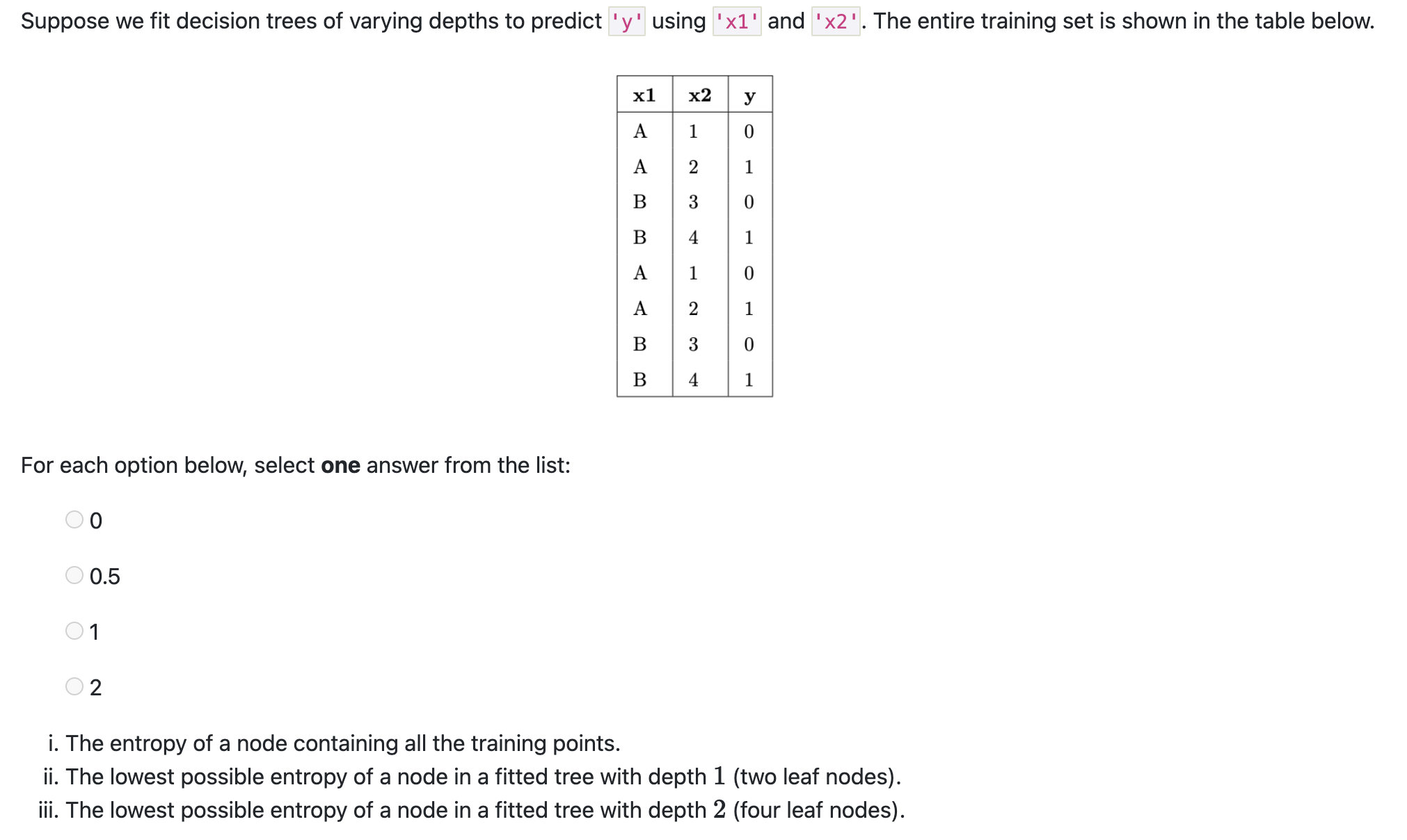
Tree depth
Decision trees are trained by recursively picking the best split until:
- all "leaf nodes" only contain training examples from a single class (good), or
- it is impossible to split leaf nodes any further (not good).
By default, there is no "maximum depth" for a decision tree. As such, without restriction, decision trees tend to be very deep.
dt_no_max = DecisionTreeClassifier()
dt_no_max.fit(X_train, y_train)
DecisionTreeClassifier()
A decision tree fit on our training data has a depth of around 20! (It is so deep that tree.plot_tree errors when trying to plot it.)
dt_no_max.tree_.max_depth
22
At first, this tree seems "better" than our tree of depth 2, since its training accuracy is much much higher:
dt_no_max.score(X_train, y_train)
0.9913194444444444
# Depth 2 tree.
dt.score(X_train, y_train)
0.765625
But recall, we truly care about test set performance, and this decision tree has worse accuracy on the test set than our depth 2 tree.
dt_no_max.score(X_test, y_test)
0.71875
# Depth 2 tree.
dt.score(X_test, y_test)
0.7760416666666666
Decision trees and overfitting
- Decision trees have a tendency to overfit. Why is that?
- Unlike linear classification techniques (like logistic regression or SVMs), decision trees are non-linear.
- They are also "non-parametric" – there are no $w^*$s to learn.
- While being trained, decision trees ask enough questions to effectively memorize the correct response values in the training set. However, the relationships they learn are often overfit to the noise in the training set, and don't generalize well.
fig
- A decision tree whose depth is not restricted will achieve 100% accuracy on any training set, as long as there are no "overlapping values" in the training set.
- Two values overlap when they have the same features $x$ but different response values $y$ (e.g. if two patients have the same glucose levels and BMI, but one has diabetes and one doesn't).
- One solution: Make the decision tree "less complex" by limiting the maximum depth.
Since sklearn.tree's plot_tree can't visualize extremely large decision trees, let's create and visualize some smaller decision trees.
trees = {}
for d in [2, 4, 8]:
    trees[d] = DecisionTreeClassifier(max_depth=d, random_state=1)
    trees[d].fit(X_train, y_train)

    plt.figure(figsize=(15, 5), dpi=100)
    plot_tree(trees[d], feature_names=X_train.columns, class_names=['no db', 'yes db'],
               filled=True, rounded=True, impurity=False)

    plt.show()


As tree depth increases, complexity increases, and our trees are more prone to overfitting. This means model bias decreases, but model variance increases.
Question: What is the "right" maximum depth to choose?
Hyperparameters for decision trees
max_depthis a hyperparameter forDecisionTreeClassifier.
- There are many more hyperparameters we can tweak; look at the documentation for examples.
min_samples_split: The minimum number of samples required to split an internal node. The larger this is, the lower our tree's model variance is – why?criterion: The function to measure the quality of a split ('gini'or'entropy').
- To ensure that our model generalizes well to unseen data, we need an efficient technique for trying different combinations of hyperparameters!
- We could write a nested
for-loop and manually callcross_val_scoreon each combination of hyperparameters, but this seems suboptimal.
- We could write a nested
Grid search
Grid search
GridSearchCV takes in:
- an un-
fitinstance of an estimator, and - a dictionary of hyperparameter values to try,
and performs $k$-fold cross-validation to find the combination of hyperparameters with the best average validation performance.
from sklearn.model_selection import GridSearchCV
The following dictionary contains the values we're considering for each hyperparameter. (We're using GridSearchCV with 3 hyperparameters, but we could use it with even just a single hyperparameter.)
hyperparameters = {
    'max_depth': [2, 3, 4, 5, 7, 10, 13, 15, 18, None],
    'min_samples_split': [2, 5, 10, 20, 50, 100, 200],
    'criterion': ['gini', 'entropy']
}
Note that there are 140 combinations of hyperparameters we need to try. We need to find the best combination of hyperparameters, not the best value for each hyperparameter individually.
np.prod([len(v) for v in hyperparameters.values()])
140
GridSearchCV needs to be instantiated and fit.
searcher = GridSearchCV(DecisionTreeClassifier(), hyperparameters, cv=5)
%%time
searcher.fit(X_train, y_train)
CPU times: user 927 ms, sys: 12.3 ms, total: 939 ms
Wall time: 939 ms
GridSearchCV(cv=5, estimator=DecisionTreeClassifier(),
             param_grid={'criterion': ['gini', 'entropy'],
                         'max_depth': [2, 3, 4, 5, 7, 10, 13, 15, 18, None],
                         'min_samples_split': [2, 5, 10, 20, 50, 100, 200]})
After being fit, the best_params_ attribute provides us with the best combination of hyperparameters to use.
searcher.best_params_
{'criterion': 'gini', 'max_depth': 4, 'min_samples_split': 50}
All of the intermediate results – validation accuracies for each fold, mean validation accuaries, etc. – are stored in the cv_results_ attribute:
searcher.cv_results_['mean_test_score'] # Array of length 140.
array([0.73, 0.73, 0.73, ..., 0.75, 0.74, 0.72])
# Rows correspond to folds, columns correspond to hyperparameter combinations.
pd.DataFrame(np.vstack([searcher.cv_results_[f'split{i}_test_score'] for i in range(5)]))
| 0 | 1 | 2 | 3 | ... | 136 | 137 | 138 | 139 | |
|---|---|---|---|---|---|---|---|---|---|
| 0 | 0.71 | 0.71 | 0.71 | 0.71 | ... | 0.70 | 0.68 | 0.71 | 0.73 |
| 1 | 0.77 | 0.77 | 0.77 | 0.77 | ... | 0.82 | 0.83 | 0.77 | 0.76 |
| 2 | 0.74 | 0.74 | 0.74 | 0.74 | ... | 0.68 | 0.72 | 0.74 | 0.73 |
| 3 | 0.70 | 0.70 | 0.70 | 0.70 | ... | 0.77 | 0.79 | 0.76 | 0.70 |
| 4 | 0.72 | 0.72 | 0.72 | 0.72 | ... | 0.70 | 0.71 | 0.72 | 0.70 |
5 rows × 140 columns
Note that the above DataFrame tells us that 5 * 140 = 700 models were trained in total!
Now that we've found the best combination of hyperparameters, we should fit a decision tree instance using those hyperparameters on our entire training set.
searcher.best_params_
{'criterion': 'gini', 'max_depth': 4, 'min_samples_split': 50}
final_tree = DecisionTreeClassifier(**searcher.best_params_)
final_tree
DecisionTreeClassifier(max_depth=4, min_samples_split=50)
final_tree.fit(X_train, y_train)
DecisionTreeClassifier(max_depth=4, min_samples_split=50)
# Training accuracy.
final_tree.score(X_train, y_train)
0.7881944444444444
# Testing accuracy.
final_tree.score(X_test, y_test)
0.765625
Remember, searcher itself is a model object (we had to fit it). After performing $k$-fold cross-validation, behind the scenes, searcher is trained on the entire training set using the optimal combination of hyperparameters.
In other words, searcher makes the same predictions that final_tree does!
searcher.score(X_train, y_train)
0.7881944444444444
searcher.score(X_test, y_test)
0.765625
Choosing possible hyperparameter values
- A full grid search can take a long time.
- In our previous example, we tried 140 combinations of hyperparameters.
- Since we performed 5-fold cross-validation, we trained 700 decision trees under the hood.
- Question: How do we pick the possible hyperparameter values to try?
- Answer: Trial and error.
- If the "best" choice of a hyperparameter was at an extreme, try increasing the range.
- For instance, if you try
max_depths from 32 to 128, and 32 was the best, try includingmax_depthsunder 32.
Key takeaways
- To efficiently find hyperparameters through cross-validation, use
GridSearchCV.
- Specify which values to try for each hyperparameter, and
GridSearchCVwill try all unique combinations of hyperparameters and return the combination with the best average validation performance.
GridSearchCVis not the only solution – seeRandomizedSearchCVif you're curious.
Question 🤔 (Answer at q.dsc80.com)
Remember, you can always ask questions at q.dsc80.com!
Random forests
Recap: Decision trees
Decision trees are trained by finding the best questions to ask using the features in the training data. A good question is one that isolates classes as much as possible (i.e., one that minimizes the entropy of the resulting child nodes).
✅ Pros:
- Relatively fast to train and make predictions.
- Making predictions: $O(\text{tree depth})$, which is usually $O(\log n)$.
- Training: see
sklearn's documentation.
- Easily interpretable.
- Robust to irrelevant features – why?
- Linear transformations on features don't affect predictions – why?
❌ Cons:
- High variance: complete tree (no depth limit) will almost always overfit!
- Aren't the best at prediction in general (sensitive to outliers and noise in the training data, not good at extrapolating outside of the training data).
sklearn's documentation provides a good overview of the pros and cons of decision trees.
Another idea for reducing decision tree variance
We've already seen two ways to reduce the variance of a decision tree:
- Control maximum depth: as
max_depthdecreases, variance decreases.
- Only split nodes if they have a certain number of points: as
min_samples_splitincreases, variance decreases.
Here's another idea: train a bunch of decision trees, then have them vote on a prediction!
- Problem: If you use the same training data, you will always get the same tree.
- Solution: Introduce randomness into training procedure to get different trees.
Idea 1: Bootstrap the training data
- We can bootstrap the training data $T$ times, then train one tree on each resample.
- Also known as bagging (Bootstrap AGgregating). In general, combining different predictors together is a useful technique called ensemble learning.
- In practice, this doesn't make decision trees different enough from one another; for instance, if you have one really important feature, it'll always be used in the first split.
Idea 2: Only use a subset of features
- At each split, take a random subset of $ m $ features instead of choosing from all $ d $ of them.
- Rule of thumb: $ m \approx \sqrt d $ seems to work well. (This is the default that
sklearnuses in the algorithm we're about to learn about.)
- Key idea: For ensemble learning, you want the individual predictors to have low bias, high variance, and be uncorrelated with each other. That way, when you average them together, you have low bias AND low variance.
- Random forest algorithm: Fit $T$ trees by using bagging and a random subset of features at each split. Predict by taking a vote from the $ T $ trees.
- Decreasing $m$ tends to decrease the correlation between the individual trees, but increases the bias and decreases the variance of the individual trees.
Example: Predicting diabetes
We'll again aim to predict whether or not someone has diabetes, but this time, we'll use all possible columns in diabetes as features, rather than just 'Glucose' and 'BMI'.
X_train, X_test, y_train, y_test = (
    train_test_split(diabetes.drop(columns=['Outcome']), diabetes['Outcome'], random_state=1)
)
from sklearn.ensemble import RandomForestClassifier
Note that the default number of trees (n_trees) is 100, but this is a hyperparameter we could tune if we'd like.
rf = RandomForestClassifier()
rf.fit(X_train, y_train)
RandomForestClassifier()
rf.score(X_train, y_train)
1.0
# Note that because random forests are _random_,
# if you re-train the model above, the test accuracy
# you get will be slightly different every time!
rf.score(X_test, y_test)
0.8072916666666666
Our random forest has both a better training accuracy and a better test accuracy than the best decision tree with a depth of 4:
dt = DecisionTreeClassifier(max_depth=4, criterion='entropy')
dt.fit(X_train, y_train)
DecisionTreeClassifier(criterion='entropy', max_depth=4)
dt.score(X_train, y_train)
0.7829861111111112
dt.score(X_test, y_test)
0.7395833333333334
Question 🤔 (Answer at q.dsc80.com)
Remember, you can always ask questions at q.dsc80.com!
Modeling using text features
news = pd.read_csv(Path('data') / 'fake_news_training.csv')
news
| baseurl | content | label | |
|---|---|---|---|
| 0 | twitter.com | \njavascript is not available.\n\nwe’ve detect... | real |
| 1 | whitehouse.gov | remarks by the president at campaign event -- ... | real |
| 2 | web.archive.org | the committee on energy and commerce\nbarton: ... | real |
| ... | ... | ... | ... |
| 658 | politico.com | full text: jeff flake on trump speech transcri... | fake |
| 659 | pol.moveon.org | moveon.org political action: 10 things to know... | real |
| 660 | uspostman.com | uspostman.com is for sale\nyes, you can transf... | fake |
661 rows × 3 columns
Goal: Use an article's content to predict its label.
news['label'].value_counts(normalize=True)
real    0.55
fake    0.45
Name: label, dtype: float64
Question: What is the worst possible accuracy we should expect from a classifier, given the above distribution?
Aside: CountVectorizer
Entries in the 'content' column are not currently quantitative! We can use the bag of words encoding to create quantitative features out of each 'content'.
Instead of performing a bag of words encoding manually as we did before, we can rely on sklearn's CountVectorizer. (There is also a TfidfVectorizer.)
from sklearn.feature_extraction.text import CountVectorizer
example_corp = ['hey hey hey my name is billy',
                'hey billy how is your dog billy']
count_vec = CountVectorizer()
count_vec.fit(example_corp)
CountVectorizer()
count_vec learned a vocabulary from the corpus we fit it on.
count_vec.vocabulary_
{'hey': 2,
 'my': 5,
 'name': 6,
 'is': 4,
 'billy': 0,
 'how': 3,
 'your': 7,
 'dog': 1}
count_vec.transform(example_corp).toarray()
array([[1, 0, 3, 0, 1, 1, 1, 0],
       [2, 1, 1, 1, 1, 0, 0, 1]])
Note that the values in count_vec.vocabulary_ correspond to the positions of the columns in count_vec.transform(example_corp).toarray(), i.e. 'billy' is the first column and 'your' is the last column.
example_corp
['hey hey hey my name is billy', 'hey billy how is your dog billy']
pd.DataFrame(count_vec.transform(example_corp).toarray(),
             columns=pd.Series(count_vec.vocabulary_).sort_values().index)
| billy | dog | hey | how | is | my | name | your | |
|---|---|---|---|---|---|---|---|---|
| 0 | 1 | 0 | 3 | 0 | 1 | 1 | 1 | 0 |
| 1 | 2 | 1 | 1 | 1 | 1 | 0 | 0 | 1 |
Creating an initial Pipeline
Let's build a Pipeline that takes in summaries and overall ratings and:
Uses
CountVectorizerto quantitatively encode summaries.Fits a
RandomForestClassifierto the data.
But first, a train-test split (like always).
from sklearn.model_selection import train_test_split
from sklearn.pipeline import Pipeline
from sklearn.ensemble import RandomForestClassifier
X = news['content']
y = news['label']
X_train, X_test, y_train, y_test = train_test_split(X, y)
To start, we'll create a random forest with 100 trees (n_estimators) each of which has a maximum depth of 3 (max_depth).
pl = Pipeline([
    ('cv', CountVectorizer()),
    ('clf', RandomForestClassifier(
        max_depth=3,
        n_estimators=100, # Uses 100 separate decision trees!
        random_state=42,
    ))
])
pl.fit(X_train, y_train)
Pipeline(steps=[('cv', CountVectorizer()),
                ('clf', RandomForestClassifier(max_depth=3, random_state=42))])
# Training accuracy.
pl.score(X_train, y_train)
0.7636363636363637
# Testing accuracy.
pl.score(X_test, y_test)
0.6927710843373494
The accuracy of our random forest is just under 73% on the test set. How much better does it do compared to a classifier that predicts "real" every time?
y_train.value_counts(normalize=True)
real    0.55
fake    0.45
Name: label, dtype: float64
# Distribution of predicted ys in the training set:
pd.set_option('display.float_format', '{:.3f}'.format) # Stops scientific notation for pandas.
pd.Series(pl.predict(X_train)).value_counts(normalize=True)
fake   0.634
real   0.366
dtype: float64
len(pl.named_steps['cv'].vocabulary_) # Lots of features!
25500
Choosing tree depth via GridSearchCV
We arbitrarily chose max_depth=3 before, but it seems like that isn't working well. Let's perform a grid search to find the max_depth with the best generalization performance.
# Note that we've used the key clf__max_depth, not max_depth
# because max_depth is a hyperparameter of clf, not of pl.

hyperparameters = {
    'clf__max_depth': np.arange(2, 200, 20)
}
Note that while pl has already been fit, we can still give it to GridSearchCV, which will repeatedly re-fit it during cross-validation.
%%time

# Takes a few seconds to run – how many trees are being trained?
from sklearn.model_selection import GridSearchCV
grids = GridSearchCV(
    pl,
    n_jobs=-1, # Use multiple processors to parallelize.
    param_grid=hyperparameters,
    return_train_score=True
)
grids.fit(X_train, y_train)
CPU times: user 617 ms, sys: 205 ms, total: 823 ms
Wall time: 5.88 s
GridSearchCV(estimator=Pipeline(steps=[('cv', CountVectorizer()),
                                       ('clf',
                                        RandomForestClassifier(max_depth=3,
                                                               random_state=42))]),
             n_jobs=-1,
             param_grid={'clf__max_depth': array([  2,  22,  42,  62,  82, 102, 122, 142, 162, 182])},
             return_train_score=True)
grids.best_params_
{'clf__max_depth': 42}
Recall, fit GridSearchCV objects are estimators on their own as well. This means we can compute the training and testing accuracies of the "best" random forest directly:
# Training accuracy.
grids.score(X_train, y_train)
0.9919191919191919
# Testing accuracy.
grids.score(X_test, y_test)
0.8614457831325302
When using the max depth above, we see ~10% better test set performance than with a max depth of 3!
Training and validation accuracy vs. depth
Below, we plot how training and validation accuracy varied with tree depth. Note that the $y$-axis here is accuracy, and that larger accuracies are better (unlike with RMSE, where smaller was better).
index = grids.param_grid['clf__max_depth']
train = grids.cv_results_['mean_train_score']
valid = grids.cv_results_['mean_test_score']
pd.DataFrame({'train': train, 'valid': valid}, index=index).plot().update_layout(
    xaxis_title='max_depth', yaxis_title='Accuracy'
)
Question 🤔 (Answer at q.dsc80.com)
Remember, you can always ask questions at q.dsc80.com!
Classifier evaluation
Accuracy isn't everything!
$$ \text{accuracy} = \frac{\text{# data points classified correctly}}{\text{# data points}} $$- Accuracy is defined as the proportion of predictions that are correct.
- It weighs all correct predictions the same, and weighs all incorrect predictions the same.
- But some incorrect predictions may be worse than others!
- Example: Suppose you take a COVID test 🦠. Which is worse:
- The test saying you have COVID, when you really don't, or
- The test saying you don't have COVID, when you really do?
- Example: Suppose you take a COVID test 🦠. Which is worse:
Repeat the previous paragraph many, many times.
One night, the shepherd boy sees a real wolf approaching the flock and calls out, "Wolf!" The villagers refuse to be fooled again and stay in their houses. The hungry wolf turns the flock into lamb chops. The town goes hungry. Panic ensues.
The wolf classifier
- Predictor: Shepherd boy.
- Positive prediction: "There is a wolf."
- Negative prediction: "There is no wolf."
Some questions to think about:
- What is an example of an incorrect, positive prediction?
- Was there a correct, negative prediction?
- There are four possibilities. What are the consequences of each?
- (predict yes, predict no) x (actually yes, actually no).
The wolf classifier
Below, we present a confusion matrix, which summarizes the four possible outcomes of the wolf classifier.

Outcomes in binary classification
When performing binary classification, there are four possible outcomes.
(Note: A "positive prediction" is a prediction of 1, and a "negative prediction" is a prediction of 0.)
| Outcome of Prediction | Definition | True Class |
|---|---|---|
| True positive (TP) ✅ | The predictor correctly predicts the positive class. | P |
| False negative (FN) ❌ | The predictor incorrectly predicts the negative class. | P |
| True negative (TN) ✅ | The predictor correctly predicts the negative class. | N |
| False positive (FP) ❌ | The predictor incorrectly predicts the positive class. | N |
| Predicted Negative | Predicted Positive | |
|---|---|---|
| Actually Negative | TN ✅ | FP ❌ |
| Actually Positive | FN ❌ | TP ✅ |
sklearn's confusion matrices are (but differently than in the wolf example).Note that in the four acronyms – TP, FN, TN, FP – the first letter is whether the prediction is correct, and the second letter is what the prediction is.
Example: COVID testing 🦠
- UCSD Health administers hundreds of COVID tests a day. The tests are not fully accurate.
- Each test comes back either:
- positive, indicating that the individual has COVID, or
- negative, indicating that the individual does not have COVID.
- What is a TP in this scenario? FP? TN? FN?
- TP: The test predicted that the individual has COVID, and they do ✅.
- FP: The test predicted that the individual has COVID, but they don't ❌.
- TN: The test predicted that the individual doesn't have COVID, and they don't ✅.
- FN: The test predicted that the individual doesn't have COVID, but they do ❌.
Accuracy of COVID tests
The results of 100 UCSD Health COVID tests are given below.
| Predicted Negative | Predicted Positive | |
|---|---|---|
| Actually Negative | TN = 90 ✅ | FP = 1 ❌ |
| Actually Positive | FN = 8 ❌ | TP = 1 ✅ |
🤔 Question: What is the accuracy of the test?
🙋 Answer: $$\text{accuracy} = \frac{TP + TN}{TP + FP + FN + TN} = \frac{1 + 90}{100} = 0.91$$
- Followup: At first, the test seems good. But, suppose we build a classifier that predicts that nobody has COVID. What would its accuracy be?
- Answer to followup: Also 0.91! There is severe class imbalance in the dataset, meaning that most of the data points are in the same class (no COVID). Accuracy doesn't tell the full story.
Recall
| Predicted Negative | Predicted Positive | |
|---|---|---|
| Actually Negative | TN = 90 ✅ | FP = 1 ❌ |
| Actually Positive | FN = 8 ❌ | TP = 1 ✅ |
🤔 Question: What proportion of individuals who actually have COVID did the test identify?
🙋 Answer: $\frac{1}{1 + 8} = \frac{1}{9} \approx 0.11$.
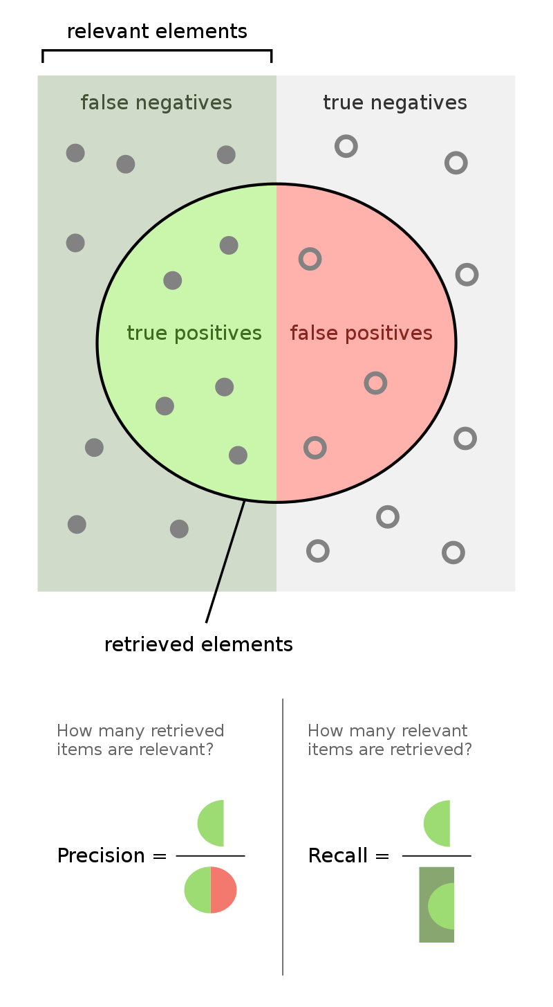
More generally, the recall of a binary classifier is the proportion of actually positive instances that are correctly classified. We'd like this number to be as close to 1 (100%) as possible.
$$\text{recall} = \frac{TP}{\text{# actually positive}} = \frac{TP}{TP + FN}$$To compute recall, look at the bottom (positive) row of the above confusion matrix.
Recall isn't everything, either!
$$\text{recall} = \frac{TP}{TP + FN}$$🤔 Question: Can you design a "COVID test" with perfect recall?
🙋 Answer: Yes – just predict that everyone has COVID!
| Predicted Negative | Predicted Positive | |
|---|---|---|
| Actually Negative | TN = 0 ✅ | FP = 91 ❌ |
| Actually Positive | FN = 0 ❌ | TP = 9 ✅ |
Like accuracy, recall on its own is not a perfect metric. Even though the classifier we just created has perfect recall, it has 91 false positives!
Precision
| Predicted Negative | Predicted Positive | |
|---|---|---|
| Actually Negative | TN = 0 ✅ | FP = 91 ❌ |
| Actually Positive | FN = 0 ❌ | TP = 9 ✅ |
The precision of a binary classifier is the proportion of predicted positive instances that are correctly classified. We'd like this number to be as close to 1 (100%) as possible.
$$\text{precision} = \frac{TP}{\text{# predicted positive}} = \frac{TP}{TP + FP}$$To compute precision, look at the right (positive) column of the above confusion matrix.
- Tip: A good way to remember the difference between precision and recall is that in the denominator for 🅿️recision, both terms have 🅿️ in them (TP and FP).
- Note that the "everyone-has-COVID" classifier has perfect recall, but a precision of $\frac{9}{9 + 91} = 0.09$, which is quite low.
- 🚨 Key idea: There is a "tradeoff" between precision and recall. Ideally, you want both to be high. For a particular prediction task, one may be important than the other.
Precision and recall
$$\text{precision} = \frac{TP}{TP + FP} \: \: \: \: \: \: \: \: \text{recall} = \frac{TP}{TP + FN}$$🤔 Question: When might high precision be more important than high recall?
🙋 Answer: For instance, in deciding whether or not someone committed a crime. Here, false positives are really bad – they mean that an innocent person is charged!
🤔 Question: When might high recall be more important than high precision?
🙋 Answer: For instance, in medical tests. Here, false negatives are really bad – they mean that someone's disease goes undetected!
Exercise
Consider the confusion matrix shown below.
| Predicted Negative | Predicted Positive | |
|---|---|---|
| Actually Negative | TN = 22 ✅ | FP = 2 ❌ |
| Actually Positive | FN = 23 ❌ | TP = 18 ✅ |
What is the accuracy of the above classifier? The precision? The recall?
After calculating all three on your own, click below to see the answers.
👉 Accuracy
(22 + 18) / (22 + 2 + 23 + 18) = 40 / 65👉 Precision
18 / (18 + 2) = 9 / 10👉 Recall
18 / (18 + 23) = 18 / 41Summary, next time
Summary
- Decision trees, while interpretable, are prone to having high variance. There are several ways to control the variance of a decision tree:
- Limit
max_depthor increasemin_samples_split. - Create a random forest, which is an ensemble of multiple decision trees, each fit to a different random resample of the training data, using a random sample of features.
- Limit
- In order to tune model hyperparameters – that is, to find the hyperparameters that (likely) maximize performance on unseen data – use
GridSearchCV. - Accuracy alone is not always a meaningful representation of a classifier's quality, particularly when the classes are imbalanced.
- Precision and recall are classifier evaluation metrics that consider the types of errors being made.
- There is a "tradeoff" between precision and recall. One may be more important than the other, depending on the task.
Next time
Next time, we'll learn about logistic regression, another powerful classification technique. We'll use it in a practical example, and focus on understanding the tradeoffs between precision, recall, and accuracy.