Hypothesis Test

Concept

Note 🌟

This page refers to the standard hypothesis test.

Key Idea

We use a hypothesis test to test whether a sample was drawn from a population.

Terminology

Hypothesis Test: A process that test whether a sample was drawn from a population, given a population distribution and a sample.

To conduct a hypothesis test:

Simulate the experiment many times under the assumption that the null hypothesis is true.
Compute a test statistic on each of the simulated samples, as well as on the observed sample.
Look at the resulting empirical distribution of test statistics and see where the observed test statistic falls. If it seems like an atypical value (too large or too small), we reject the null hypothesis; otherwise, we fail to reject the null.

Code Example 1 (Difference)

1. State the question/hypothesis

Hypotheses

We will test the following pair of hypotheses at the standard p = 0.05 significance level.

Null Hypothesis: The proportion of "white" dogs among dogs is equal to the proportion of "white" pets in the overall population.
Alternative Hypothesis: The distribution of "white" dogs among dogs is greater than the proportion of "white" pets in the overall population.

Since the alternative hypothesis is of the form "A is greater than B," the test statistic should measure signed difference rather than absolute difference.

$\therefore$ We use the difference in proportions of white dogs among dogs and white pets in the overall poplulation as the test statistic.

2. Calculate the overall proportion

We first compute the proportion of white pets in the overall population, which will be used for calculating the test statistic.

#Method 1: Obtain a series of boolean values (1s and 0s), and calculate the mean
overall_prop = (full_pets.get('Color')=='white').mean()

#Method 2: Query the DataFrame and obtain the proportion by using .shape[0]
#overall_prop = full_pets[full_pets.get('Color')=='white'].shape[0]/full_pets.shape[0]

overall_prop

0.2631578947368421

3. Create a function to calculate test statistic

Create a function to calculate the test statistic during every trial of our hypothesis test.

def difference_in_proportions(dogs_prop, overall_prop):
    """
    Calculate the difference in proportions of white dogs among dogs and white pets in the overall population.
    ---
    Input:
        dogs_prop: the proportion of white dogs among all dogs.
        overall_prop: the proportion of white pets in the overall population.
    ---
    Output:
        The difference in proportions of white dogs among dogs and white pets in the overall population.
    """
    return dogs_prop - overall_prop

Note: Although we can simply do this in the for-loop shown in the next step, we can practice good coding habits by separating our code into readable bits!

4. Compute the observed statistic

# Query the DataFrame to only include dogs
dogs_df = full_pets[full_pets.get('Species') == 'dog']
# Compute the observed proportion of white dogs among all dogs
obs_dogs_prop = (dogs_df.get('Color') == 'white').mean()
# Calculate the observed statistic
observed_stat = difference_in_proportions(obs_dogs_prop, overall_prop)
observed_stat

0.18128654970760233

5. Simulate the hypothesis test under the null hypothesis

n = 500 # Number of simulations.
test_statistics = np.array([]) # Array to keep track of the test statistic for each iteration.

# Calculte the smaple size (number of dogs)
sample_size = dogs_df.shape[0]

# Under the null hypothesis, proportion of "white" dogs among dogs is equal to the proportion of white pets among the overall population
model_proportions = np.array([obs_dogs_prop, 1-obs_dogs_prop]) 

for i in np.arange(n): # Run the simulation `n` number of times
    
    # 1. Simulate the dogs distribution
    # Calculate the the proportion of white dogs among all dogs.
    simulation_proportion = np.random.multinomial(sample_size, model_proportions)[0] / sample_size
    
    # 2. Compute the test statistic
    test_stat = difference_in_proportions(simulation_proportion, overall_prop)

    # 3. Save the result
    test_statistics = np.append(test_statistics, test_stat)

This code will run the hypothesis test 500 times, but a different reasonable number can be used instead. It is crucial to keep track of the test statistic each time our for-loop runs so that the number of simulated values can be stored.

6. Conclusion

p_value = np.count_nonzero(test_statistics >= observed_stat) / n

print("The observed value of the test statistic is:", observed_stat)
print("The p-value is:", p_value)

The observed value of the test statistic is: 0.18128654970760233
The p-value is: 0.616

Using a significance level of 0.05:

Conclusion

Under the null hypothesis, there is a sufficiently large probability of seeing a difference greater than the observed value. The data are consistent with the null hypothesis.
Since our p-value is greater than 0.05, we fail to reject the null hypothesis.

7. Extra

Let's see how our observed statistic compares to the overall simulated values!

# Create the histogram.
bpd.DataFrame().assign(test_statistics=test_statistics).plot(kind='hist', bins= 10, density=True, ec='w')
# Don't worry about these lines - you won't need to know it for this course!
plt.axvline(x=observed_stat, c='black', linewidth=4);
yticks = plt.gca().get_yticks()
plt.yticks(yticks, np.round(yticks * 0.1, 2))
plt.show()

Distribution

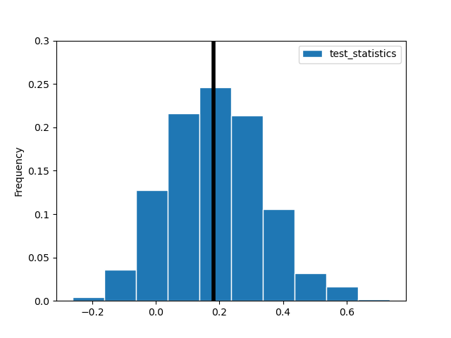
From this graph, we can see that more than half of the data are to the right of the black vertical line (our observed statistic), meaning we have a relatively high p-value!

Code Example 2 (TVD)

1. State the question/hypothesis

We found that the color distribution of dogs seems different from that of all pets.

Index	Pets_Dist	Dogs_Dist
black	0.53	0.44
golden	0.21	0.12
white	0.26	0.44

To see whether this difference is due to random chance, we will test the following pair of hypotheses at the standard p = 0.05 significance level.

Hypotheses

Null Hypothesis: The color distribution of dogs is the same as the color distribution of pets.
Alternative Hypothesis: The color distribution of dogs is different from the color distribution of pets.

Since we are comparing two categorical distributions, we use Total Variation Distance (TVD) between the two distributions as our test statistic.

2. Create a function to calculate test statistic (TVD)

Create a function to calculate the test statistic during every trial of our hypothesis test.

def total_variation_distance(dist1, dist2):
    '''Computes the TVD between two categorical distributions, 
       assuming the categories appear in the same order.'''
    return np.abs((dist1 - dist2)).sum() / 2

3. Compute the observed statistic

pets_color_dist = np.array([0.53, 0.21, 0.26])
dogs_color_dist = np.array([0.44, 0.12, 0.44])
observed_tvd = total_variation_distance(dogs_color_dist, pets_color_dist)
observed_tvd

0.18

4. Simulate the hypothesis test under the null hypothesis

n = 5000 # Number of simulations.
tvds = np.array([]) # Array to keep track of the test statistic for each iteration.

# Get sample df (dogs df)
dog_df = full_pets[full_pets.get('Species') == 'dog'] 

# Calculte the smaple size (number of dogs)
sample_size = dog_df.shape[0]

for i in np.arange(n): # Run the simulation `n` number of times
    
    # 1. Simulate the color distribution of dogs.
    # Under the null hypothesis, color distribution of dogs should be equal to the color distribution of pets among the overall population
    sample_distribution = np.random.multinomial(sample_size, pets_color_dist) / sample_size

    # 2. Compute the test statistic (TVD)
    new_tvd = total_variation_distance(sample_distribution, pets_color_dist)

    # 3. Save the result
    tvds = np.append(tvds, new_tvd)

This code will run the hypothesis test 5000 times, but a different reasonable number can be used instead. It is crucial to keep track of the test statistic each time our for-loop runs so that the number of simulated values can be stored.

5. Conclusion

p_value = np.count_nonzero(tvds >= observed_tvd) / n

print("The observed value of the test statistic is:", observed_tvd)
print("The p-value is:", p_value)

The observed value of the test statistic is: 0.18
The p-value is: 0.4972

Using a significance level of 0.05:

Conclusion

Under the null hypothesis, there is a sufficiently large probability of seeing a difference greater than the observed value. The data are consistent with the null hypothesis.
Since our p-value is greater than 0.05, we fail to reject the null hypothesis.

6. Extra

Let's see how our observed statistic compares to the overall simulated values!

# Create the histogram.
bpd.DataFrame().assign(tvds=tvds).plot(kind='hist', density=True, bins=20, ec='w', figsize=(10, 5), title='Empirical Distribution of TVD Between Pets Colors and Dogs Colors')
# Don't worry about these lines - you won't need to know it for this course!
plt.axvline(observed_tvd, color='black', linewidth=4, label='Observed Statistic')
plt.legend();

Distribution

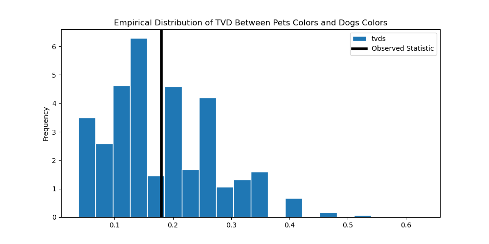
From this graph, we can see that almost half of the data are to the right of the black vertical line (our observed statistic), meaning we have a relatively high p-value!

Concept​

Code Example 1 (Difference)​

1. State the question/hypothesis​

2. Calculate the overall proportion​

3. Create a function to calculate test statistic​

4. Compute the observed statistic​

5. Simulate the hypothesis test under the null hypothesis​

6. Conclusion​

7. Extra​

Code Example 2 (TVD)​

1. State the question/hypothesis​

2. Create a function to calculate test statistic (TVD)​

3. Compute the observed statistic​

4. Simulate the hypothesis test under the null hypothesis​

5. Conclusion​

6. Extra​

Concept

Code Example 1 (Difference)

1. State the question/hypothesis

2. Calculate the overall proportion

3. Create a function to calculate test statistic

4. Compute the observed statistic

5. Simulate the hypothesis test under the null hypothesis

6. Conclusion

7. Extra

Code Example 2 (TVD)

1. State the question/hypothesis

2. Create a function to calculate test statistic (TVD)

3. Compute the observed statistic

4. Simulate the hypothesis test under the null hypothesis

5. Conclusion

6. Extra