Standard Units, Correlation, Regression

Concept

Key Idea

We use regression to make predictions about the data (based on the correlation between two variables in standard units).

Terminology

Association: Any relationship or link between two variables in a scatter plot.

• Positive association: as one variable increases, the other tends to increase.
• Negative association: as one variable increases, the other tends to decrease.

Correlation coefficient $r$: The correlation coefficient, $r$, of two variables $x$ and $y$ measures the strength of the linear association between them (how clustered points are around a straight line).

• $r$ is always between -1 and 1.

---

Formulas

Standard Units

Standardize your units to compare two variables with different units (ex. height and weight).

$x_{i(su)}=\dfrac{x_{i}-\textnormal{mean of $x$}}{\textnormal{SD of $x$}}$

variables

• $x_{i}$ = value (in original units) from column x.
• $x_{i(su)}$ = value of $x_{i}$ converted to standard units.

def standard_units(col):
    """
    Standardizes the units of a column.
    """
    return (col - col.mean()) / np.std(col)

Regression Line

A line used to make predictions about the value of y based on the correlation coefficient and the value of x.

• Both variables are measured in standard units.
• Always predicts that $y$ will be closer to the average than $x$, the regression to the mean effect.

$\textnormal{predicted y}_{i(su)} = r\cdot x_{i(su)}$

variables

• $x_{i(su)}$ = value of $x_{i}$ converted to standard units.
• $r$ = correlation coefficient, the strength of the linear association between $x$ and $y$.

def calculate_r(df, x, y):
    """
    Returns the average value of the product of x and y, 
    when both are measured in standard units.
    """
    x_su = standard_units(df.get(x))
    y_su = standard_units(df.get(y))
    return (x_su * y_su).mean()

Converting to Original Units

Finding the slope and intercept of the regression line in original units.

$\dfrac{\textnormal{predicted } y - \textnormal{mean of }y}{\textnormal{SD of }y} = r \cdot \dfrac{x - \textnormal{mean of } x}{\textnormal{SD of }x}$

Re-arranged to the form $\textnormal{predicted } y = mx + b$

• $m = r \cdot \dfrac{\textnormal{SD of } y}{\textnormal{SD of }x}$

• $b = \textnormal{mean of } y - (m \cdot \textnormal{mean of } x)$

note

• $r$, mean of x, mean of y, SD of x, and SD of y are constants.
• if you have a DataFrame with two columns, you can determine all 5 values.

def slope(df, x, y):
    """
    Returns the slope of the regression line between columns x and y in df (in original units).
    """
    r = calculate_r(df, x, y)
    return r * np.std(df.get(y)) / np.std(df.get(x))

def intercept(df, x, y):
    """
    Returns the intercept of the regression line between columns x and y in df (in original units).
    """
    return df.get(y).mean() - slope(df, x, y) * df.get(x).mean()

---

Code Example

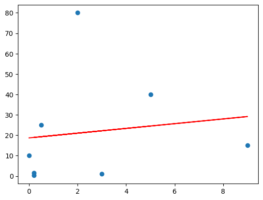
Predicting pet weight using the regression line of the Age and Weight columns.

Method 1: Using SD and Mean

Convert Age values into standard units, find SD and mean of Weight.

x_su = standard_units(full_pets.get('Age')) # series of floats ('Age' values in standard units)
y_sd = np.std(full_pets.get('Weight'))
y_mean = full_pets.get('Weight').mean()

print("SD of y:", y_sd)
print("Mean of y:", y_mean)

Plug into $\textnormal{predicted y}_{i(su)} = r\cdot x_{i(su)}$ and convert to original units.

def predict_weight():
    # Predicts the weight of a pet that is 'age' years old.
    predicted_y_su = r * x_su
    return predicted_y_su * y_sd + y_mean

This function returns an array of predicted Weight values.

Method 2: Slope-intercept Form

Calculate the correlation coefficient, slope, and intercept of the regression line.

r = calculate_r(full_pets, 'Age', 'Weight')
m = slope(full_pets, 'Age', 'Weight')
b = intercept(full_pets, 'Age', 'Weight')

print("Correlation coefficient (r):", np.round(r, 3))
print("Slope of regression line:", np.round(m, 3))
print("Intercept of regression line:", np.round(b, 3))

Correlation coefficient (r): 0.134
Slope: 1.162
Intercept: 18.704

def predict_weight2(age):
    # Predicts the weight of a pet that is 'age' years old.
    return m * age + b

Apply function to Age values for an array of predicted Weight values:

all_predictions = np.array([])

for age in full_pets.get('Age').values:
    all_predictions = np.append(all_predictions, predict_weight2(age))

Plot the regression line

plt.scatter(x=full_pets.get('Age'), y=full_pets.get('Weight'))
plt.plot(full_pets.get('Age'), all_predictions, color='red')
# or plt.plot(full_pets.get('Age'), predict_weight(), color='red')

---

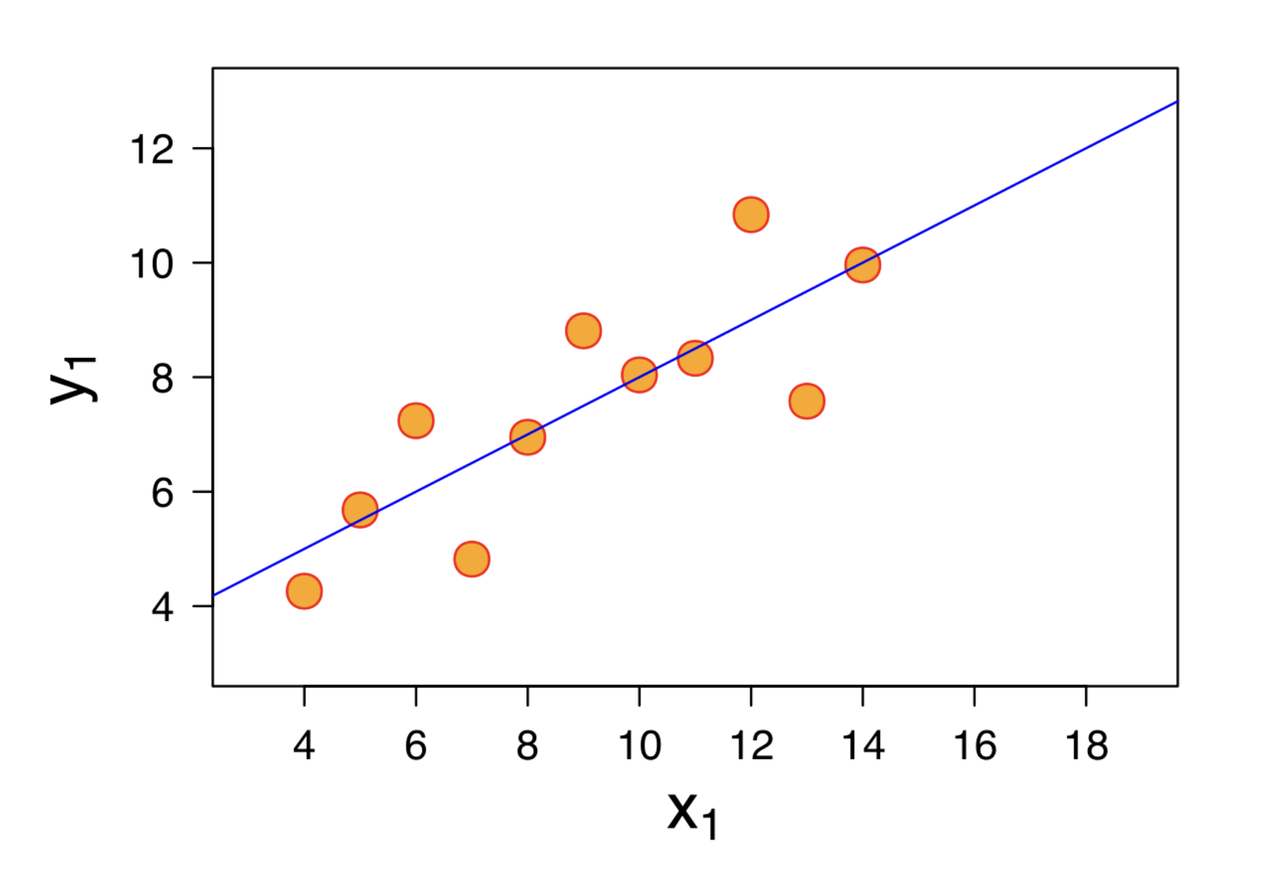
Residuals

Key Idea

If there is no pattern in a residual plot (patternless "cloud"), the regression line is a good linear fit.

Terminology

Errors: Difference between the actual and predicted values.

• $\textnormal{error} = \textnormal{actual } y - \textnormal{predicted } y$
• Any set of predictions have errors.

Residuals: Errors when using a regression line.

• $\textnormal{residual} = \textnormal{actual } y - \textnormal{predicted } y \textnormal{ by regression line}$
• There is one residual corresponding to each data point $(x, y)$ in the dataset.

Residual plots: The scatter plot with the $x$ variable on the $x$-axis and residuals on the $y$-axis.

• Residual plots describe how the error in the regression line's predictions varies.
• The correlation $r$ does not tell the full story.

Patternless "cloud" example from Anscombe's quartet:

---

Problems or suggestions about this page? Fill out our feedback form.