Spread of a Distribution

Concept

Key Idea

The Chebyshev's Inequality implies that no matter what the distribution looks like, a significant portion of the data will lie within a certain number of standard deviations from the mean. These percentages provide a way to understand the spread and variability of data even when the exact distribution is unknown.

Terminology

Standard Deviation(std): a measure of the amount of deviation in a set of values.

• Variance is the average squared deviation from the mean.
• Standard Deviation is the square root of the variance.

Chebyshev’s Inequality: Chebyshev’s Inequality states that in any dataset, at least $1 - \frac{1}{z^2}$ of the data falls within z SDs of the mean.

Formulas

Standard Deviation

$SD = \sqrt{\frac{(x_1 - mean)^2 + \cdots + (x_n - mean)^2}{n}}$

variables

• $x_{i}$ = value (in original units) from column x.

# use np to calcualte standard deviation: 
weights = full_pets.get('Weight')
standard_deviation = np.std(weights, ddof=0)

# how to implement the standard deviation formula
mean = weights.mean()
numerator = 0
for value in weights.values:
    numerator += (value - mean) ** 2
variance = numerator / (full_pets.shape[0])
standard_deviation2 = variance ** 0.5 
standard_deviation2

Chebyshev’s Inequality

Range	All Distributions	Normal Distribution
mean ± 1 SD	at least 0%	about 68%
mean ± 2 SD	at least 75%	about 95%
mean ± 3 SD	at least 88%	about 99.73%

variables

• The Chebshev's Inequality: Applies to all distributions, providing a lower bound on the proportion of data within k standard deviations from the mean.
• The true proportion of values within 𝑧 SDs of the mean may be larger than $1 - \frac{1}{z^2}$, depending on the distribution.
• Normal Distribution: Provides specific and tighter estimates because it assumes a particular symmetrical and bell-shaped distribution. These estimates are higher than the lower bounds provided by Chebyshev's Inequality because they take advantage of the normal distribution's properties.

Chebyshev’s Inequality visualized on a normal distribution

note

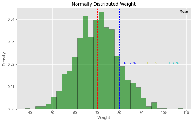
The graph above illustrates the distribution of weights sampled from a normal distribution with a mean of 70 and a standard deviation of 10. The dashed lines represent one, two, and three standard deviations from the mean, providing insight into the spread of data around the central tendency.

Annotations on the plot indicate the actual proportion of data within each standard deviation range: around 68.6% of data are within 1 std, 95.6% of data are within 2stds, 99.7% of data are within 3 stds. This aligns with the expected percentages for a normal distribution.

Chebyshev’s Inequality visualized on a non-normal distribution

note

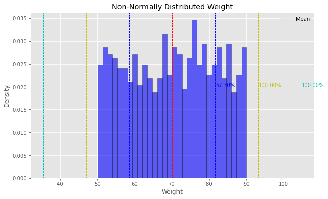
The graph above illustrates the distribution of weight values intentionally chosen to be non-normally distributed. Annotations on the plot indicate the actual proportion of data within each standard deviation range: roughly 57.3% of data fall within 1 standard deviation, while all data points fall within 2 and 3 standard deviations.

Despite the deviation from normality, Chebyshev's Inequality still applies, providing a conservative estimate of the proportion of data within a certain number of standard deviations from the mean.