Observed & Test Statistic

Concept

Terminology

Experiment: A process whose outcome is random.

• Example: Flipping 100 coins.

Observed Statistic: A statistic computed from the observed data.

• Example: The number of heads observed.

Test Statistic: A statistic computed from a sample generated under the assumption that the null hypothesis is true.

• Think of the test statistic a number you write down each time you perform an experiment.
• The test statistic should be such that high observed values lean towards one hypothesis and low observed values lean towards the other.

Common Test Statistics 🌟

1. Absolute Difference

Absolute difference in group mean/median/number of times a certain event happens.

• ✅ Used for measuring how different two numerical distributions are, and when the alternative hypothesis is not equal to. For example, "the coin is biased" or "the probability of tossing a head is 0.5".
• 💻 Example of using absolute difference as the test statistic in a permutation test.

2. Difference

Difference in group mean/median/number of times a certain event happens.

• ✅ Used for measuring how different two numerical distributions are, and the alternative hypothesis is less than or greater than. For example, "the coin is biased towards heads" or "the probability of tossing a head is greater then 0.5".
• 💻 Example of using difference as the test statistic in a hypothesis test.

3. Total Variation Distance (TVD)

A test statistic that quantifies how different two categorical distributions are by calculating the sum of the absolute differences of their proportions, all divided by 2.

• ❌️ The TVD is not used for permutation tests.
• ✅ Used for assessing whether an "observed sample" was drawn randomly from a known categorical distribution.
• 💻 Example of using TVD as the test statistic in a hypothesis test.

#code implementation
def tvd(dist1, dist2):
    '''Computes the TVD between two categorical distributions, 
       assuming the categories appear in the same order.'''
    return np.abs(dist1 - dist2).sum() / 2

note

3 Ways of Manually Computing TVD: 🧮

Assume $P$ is the first distribution and $Q$ is the second distribution, and the categories appear in the same order.

1. Follow the Definition: Calculate the sum of the absolute differences of the proportions of the two distributions $P$ and $Q$, all divided by 2.

2. Sum of Positive Differences: Add only the values where the first distribution $P$ is greater than the second distribution $Q$. This essentially sums the excessive probabilities in one distribution over the other.

3. Sum of Negative Differences: Add only the absolute values where the first distribution $P$ is less than the second distribution $Q$. This can also be interpreted as adding only the values where the second distribution $Q$ is greater than the first distribution $P$.

Any of the three methods can be the optimal choice depending on specific distributions.

Example 🌟

Let's use an example to show how TVD can be computed in three ways.

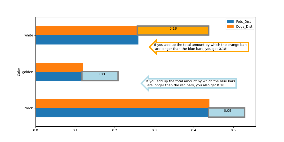
In the full_pets DataFrame, we found that the color distribution of dogs seems different from that of all pets. Let's compute the TVD between the two distributions Pets_Dist and Dogs_Dist.

Index	Pets_Dist	Dogs_Dist
black	0.53	0.44
golden	0.21	0.12
white	0.26	0.44

1. Follow the Definition

$$\begin{align*} \text{TVD} &= \frac{1}{2}(|0.53-0.44|+|0.21-0.12|+|0.26-0.44|) \\ &= \frac{1}{2}(0.09+0.09+0.18) \\ &= 0.18 \end{align*}$$

2. Sum of Positive Differences & 3. Sum of Negative Differences Assume Pets_Dist is the first distribution $P$, and Dogs_Dist is the second distribution $Q$,

Then,

$$\begin{align*} \text{TVD} &= \text{Sum of positive differences} \\ &= \text{Adding up the excessive blue bars} \\ &= (0.53-0.44)+(0.21-0.12) \\ &= 0.09+0.09 \\ &= 0.18 \end{align*}$$$$\begin{align*} \text{TVD} &= \text{Sum of negative differences} \\ &= \text{Adding up the excessive orange bar} \\ &= |0.26-0.44| \\ &= 0.18 \end{align*}$$

In this example, sum of negative differences is the fastest way to compute TVD, but it is not always optimal. Any of the three methods can be the optimal choice depending on specific distributions.